Turnstile Monitoring
In this article we’ll configure a dashboard for monitoring traffic through, and the capacity vs. occupancy of, a room. To set this up, we’ll be adding a 2-Channel Counter to our wireless sensor network (WSN), if this is your first sensor that’s ok too, I’ll cover the extremely short setup instructions for the WSN in the next section! If you don’t happen to have a convention center with turnstiles set up for testing, that’s also not a problem! Not to give away company secrets, but I’m using a couple of momentary buttons to build out the application on my desk since my boss wouldn’t spring for the optical turnstiles I asked for.
All joking aside, these sensors are extremely simple to use, and our platform of choice for this article, Node-RED, is a remarkably powerful tool for visualizing elegant UI elements quickly, and building complex logic through a flow builder with little or no actual code. If you’ve never seen Node-RED, you’re in for a treat!
By the time you’ve finished with this article, I hope you’ll be as excited as we are about the possibilities that the Industrial Internet represents, and the ease with which even someone just stepping into this arena can get up and running.
Node-RED is a cross-platform, flow based development tool that is built on NodeJS. It can be used (and we have tested it on) Mac, Windows and Linux.
Getting Set Up
Building the Wireless Sensor Network
If you’re new to the Industrial IoT scene this can sound daunting, even if you grew up programming your parents VCR, there is something about wireless networks that people see as mysterious and complicated. Fortunately, nothing could be further from the truth.
Step 1: Plug your router in to your computer with the provided USB cable.
Step 2: Attach the antenna to the sensor.
(If you are using a power supply, can skip step 3)
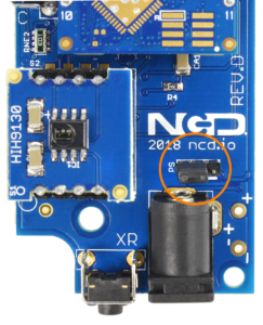
Step 3: If you plan to use battery power, remove the enclosure cover from your sensor, and move the jumper in the picture to the pins furthest away from “PS”.
Step 4: Eat a cookie, you have just successfully set up a Wireless Sensor Network!
Installing Node-RED
Seeing no need to reinvent the wheel, I’ll point you to the excellent documentation already available for Installing Node-RED.
Once that’s done, you’ll need to enter your command line, or Power Shell for Windows users, navigate to the directory Node-RED is installed in (usually ~/.node-red), and type “npm i ncd-red-wireless node-red-dashboard“. This will install the nodes required to receive data from your wireless sensors and complete this tutorial.
After the packages have finish installing, you can start Node-RED. Depending on your version the command will either be “node-red-start” or just “node-red”. You should see a message in the output like “Server now running at http://127.0.0.1:1880/”. In most cases you can just open a browser and navigate to “http://localhost:1880”. If you are on a Raspberry Pi, replace “localhost” with the IP address of the Pi.
If you're new to Node-RED, be sure to check out our Node-RED Reference post to get a head start on understanding all the terms, and nodes, used in this article.
Creating the Flow
Adding the Wireless Nodes
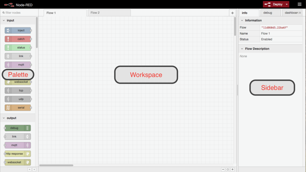
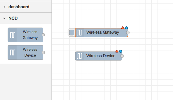
When you installed the “ncd-red-wireless” package, it added 2 new nodes to your “palette” (the name for the left-hand sidebar). These can be found under the “NCD” header. While not required, I always add one Wireless Gateway node to each flow (just drag it from the palette to the grid), this makes it easier should you need to configure the sensor or see unfiltered data coming into the router, you’ll only need one of these regardless of the number of sensors you use in your flow, it primarily gives you quick access to a couple of settings on the router.
Next you’ll need a Wireless Device node. This node serves a double purpose, it reports telemetry, and it allows you to configure the sensor, which I’ve explained in this brief tutorial.
Configuring The Nodes
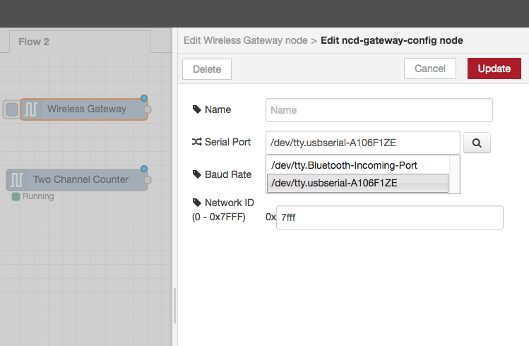
To get data from the sensor to Node-RED we use a router which you should already have connected. The sensor reports to the router, and the router reports through the USB port to your computer. Double click on a the Wireless Gateway node to open its edit panel, then click on the pencil icon next to “Serial Device” (you can ignore the “Serial Device for Config”) to open the dialog shown here. You can click the magnifying glass to discover and select your router. For a normal set up this is all that is required, the Baud Rate and Network ID are preset at the factory defaults for the devices, and should only need to be changed for advanced use cases.
After you’ve set your serial device, click update, then done. Double click on other node, you’ll now see the device you just selected in the drop down list for Serial Device, choose it, then select “Two Channel Counter” under Sensor Type. You are now ready to receive data.
Checking the Data
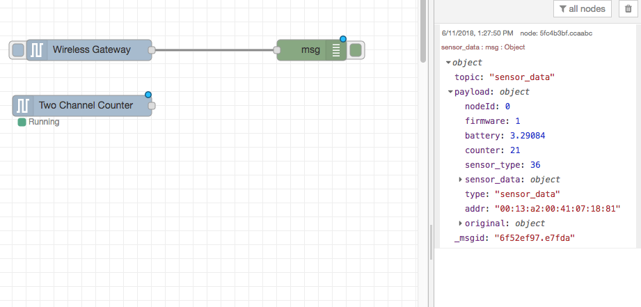
The absolute fastest way to see data coming in is using the Debug node. This node in its default configuration simply outputs the payload to the debug tab. I usually recommend wiring one of these up early in the process so you can double check the data structure you are working with, the best place to put it is on the Wireless Gateway node as shown here. This node outputs exhaustive data about the incoming transmission. The Wireless Device node will output a payload that matches the “sensor_data” property on the gateway payload. You’ll need to “deploy” your flow before you can see the debug information, once you’ve done that, clicking the RST button on the sensor will force a check in.
Sometimes you need your sensors to check in more frequently than every 10 minutes, learn how to use Node-RED to configure your sensors in this quick tutorial!
Preparing the Data
The Capacity Data
As it is, the sensor data is in a pretty simple format, which is good, but usually it needs some tweaking to get it to work well with the UI elements provided by the node-red-dashboard package. In order to change the data, we’re going to use… drumroll please… a Change node! The change node allows you to move, set, delete, or change properties of the message object without writing any code. We’re going to first build a change node to tell us the difference between the 2 channel counts. For this application that effectively means the capacity of the room. Drag a change node onto your workspace and double click on it. This change is relatively simply once you have an understanding of the underlying JSON format of the message objects.
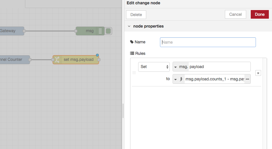
To access a property of an object in javascript we use a dot (.), so to get the payload of a message we would type msg.payload, and to get a property (say counts_1) of that payload, we again use a dot msg.payload.counts_1. In the change node edit tab, we’re going to switch the first dropdown from “Set” to “Change”, leave the msg.payload option as it is, and then next to “to” click on msg., from the dropdown select J: expression, this allows you to use a JSONata expression to set the value. This is actually pretty simple, and we won’t go into the full power of that expression language, just type msg.payload.counts_1 - msg.payload.counts_2 into the textfield. This will set the msg.payload to the result of that simple math equation. Click “Done” and draw a wire from the Two Channel Counter node to the newly created change node.
The Historical Data
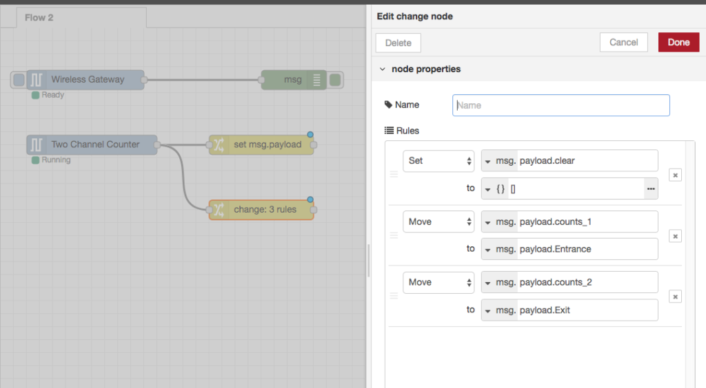
Next let’s get the data ready for our historical bar chart. Grab another change node and drag it below the first. We’re going to use 3 rules on this one, you can add new rules using the “+add” button at the bottom of the settings form. With the first rule we are going to add a property to the payload called “clear”, by default, the dashboard chart nodes aggregate the data that comes in, since these are counters the data is already aggregated, so we actually need to remove previous values from the chart before we add the new ones. So add .clear after payload in the first field, in the second field, change the msg.drop down to {} JSON, and add some empty square brackets ([]) into the field next to it.
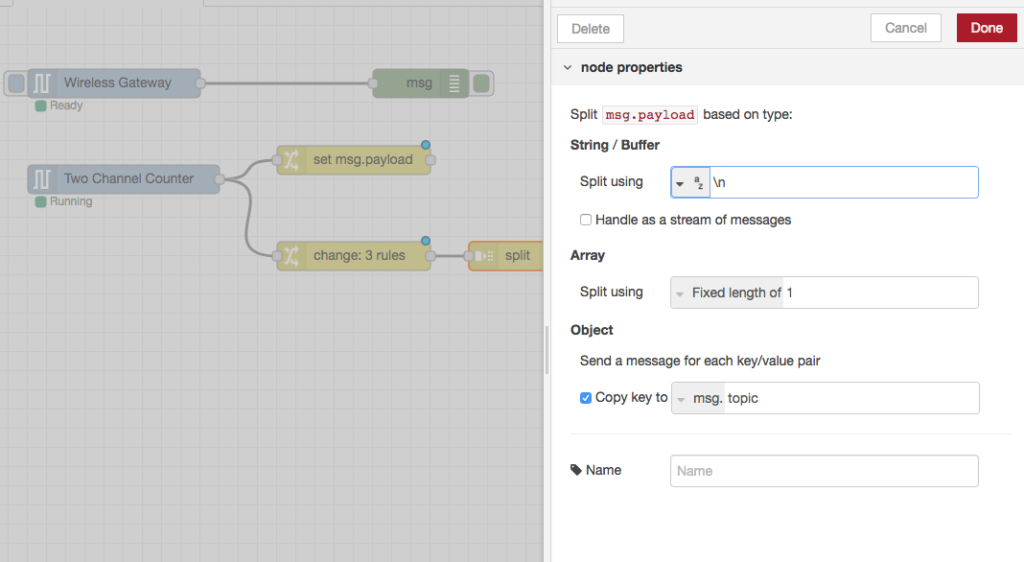
In the second set of fields change Set to Move, and type .counts_1 after payload in the first field, in the second field add .Entrance after payload. This does exactly what you’d expect, it moves the property so it has a new name, and we’ll repeat it in the next rule. Again, change Set to Move, this time add counts_2 after payload, and in the next field add .Exit after payload. Click “Done” and draw another wire from the Two Channel Counter node, this one connecting to this new change node. Now that we’ve done this, we actually need our payload to be split into multiple payloads in order for the chart to interpret it properly. This is very simple, grab a “split” node and move it over to the right of the last change node, double click on it and check the box toward the bottom of the form next to “Copy key to msg.topic”. That’s it, click Done, and draw a wire from the last change node to this split node.
The Battery Data
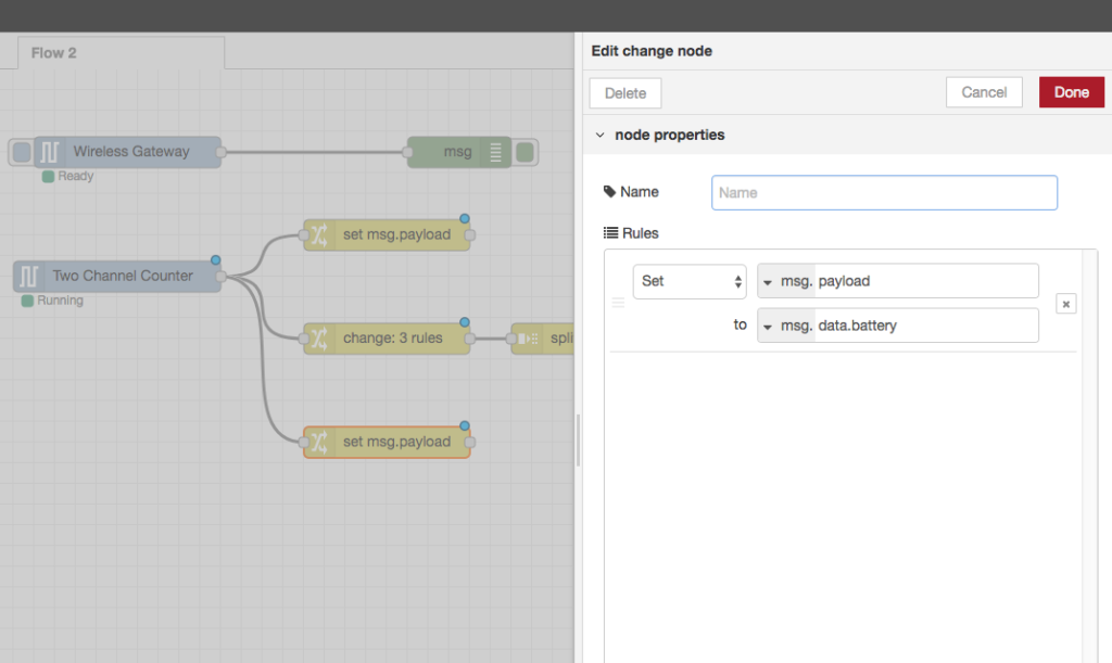
Finally, let’s add one more change node, this will change the payload so it contains the current battery level for the sensor. If you are powering your sensor with an AC power supply this isn’t necessary, but it also won’t hurt anything, and helpfully you’ll see that your battery is full! In the newest change node, leave the operation as Set, and in the to field type msg.data.battery. Wire this up to the Two Channel Counter node just like the last two, and you’re done. Now we have all of the data ready to be passed easily into the UI nodes provided from a dashboard! If you want to see it, you can drag any of the outputs to your debug node and click “Deploy”, click RST on your sensor, and see the messages rolling through. You should see 1 entry in the debug log from the first change node, 3 from the second and 1 from the 3rd. If you have them all wired to the debug node along with the gateway, that should make for a total of 5 messages with each transmission..
Node-RED is compatible with many 3rd party APIs, including popular cloud services like AWS, Azure, and Losant. Local access and control is just the tip of the iceberg!
Displaying the Data
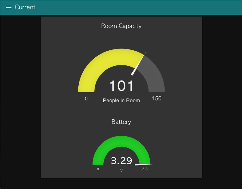
Current Capacity
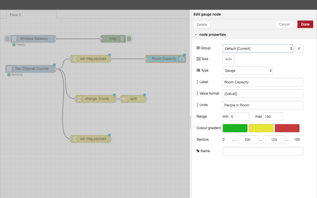
Now that the data is in the correct format, we can set up the dashboard nodes! You can find these under (surprise!) the Dashboard header in your palette. Grab a “gauge” node, move it to the right of the first change node we built, and double click on it. Click on the pencil icon next to the “group” field, then the pencil icon next to the “tab” field, change the name to “Current”. This tab will house our current sensor readings, click “Update” and “Update” again and you will be back to the gauge setting panel. You can use your own settings here, for me I assumed a maximum capacity of 150 so I set the range values to min 0, max 150. I also changed the Label to “Room Capacity” and the Units to “People in Room”. That’s all you need, click done and wire this up to the change node.
Historical Data
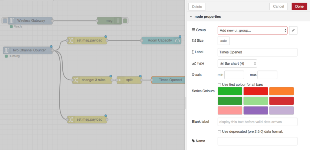
Next let’s set up a bar chart so we can see how many people have actually entered and exited the room, grab a chart node and move it to the right of the split node you added earlier. Double click on it, change the Group to “Add new ui_tab..” and click the pencil next to it, change the drop down next to “Tab” to “Add new ui_tab…”, and click the pencil. In the Name field type “History”, then click “Add” and “Add” again to bring you back to the settings tab. Change the Label to “Times Opened” and the Type to “Bar Chart (H)”. Click done and wire it up to the split node. When we moved the payload properties earlier and then split the object, the keys became the labels for this chart, so there is no need to add them.
Battery Level
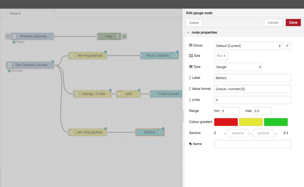
Last up we need to display the battery level, I usually just use another gauge for this, so drag one out to the right of the remaining change node and double click it. Change the Group to “Default [Current]” and the Label to “Battery”. Set the units to “V”, and since we know our max voltage is 3.3, set the max range to 3.3. You’ll notice in the screenshot that I have changed the Value format of this node, the dashboard package allows you to use Angular filters to help format the displayed data, this is particularly helpful if you don’t need to display your battery level to the 10th decimal, change {{value}} to {{value | number: 2}}, this sends the value through an angular filter and rounds it to 2 decimal places. The only other change I made here was to set the Size, click on the “auto” next to Size and drag it so it fills the width, but is only 4 cells tall, this makes the gauge a little smaller, but still centered. Click Done and wire it up!
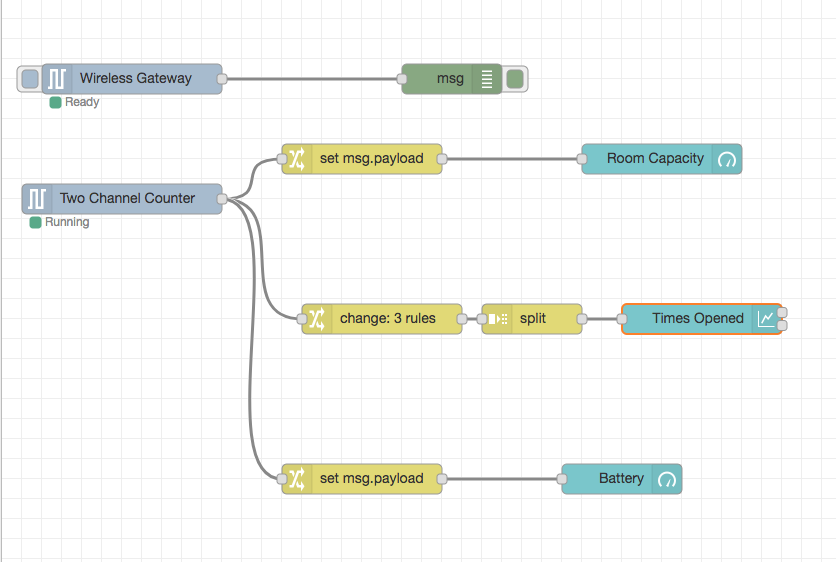
A Finished Flow
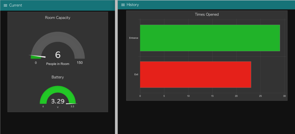
If you’ve done everything correctly you should be able to click “Deploy” and see a happy message at the top of the workspace the says “Successfully Deployed”! All the little blue dots that are remaining on your screen will have disappeared and you’ll be able to visit the dashboard. You can either open a new browser tab and navigate directly to it at http://localhost:1880/ui (or http://<ip_address>:1880/ui), or you can check out the dashboard panel in the sidebar, and use the link in the top right of the tab to open it in a new window. If you don’t see a dashboard tab, you can view it by going to the menu on the top right of the page, hovering over “View” and clicking “Dashboard”. You may notice that the dashboard is white and blue, rather than the super cool dark theme in the screenshots of this post… you can remedy that by going to the dashboard panel, clicking the “Theme” tab, and changing the Style to “Dark”. When viewing the dashboard you can toggle between the “Current” and “History” tabs we created via the hamburger menu on the top left!
The Final Product
Thanks for Reading!
I hope you’ve found this tutorial helpful, and that you continue to build using Node-RED and these amazing sensors. If this whole thing still feels overwhelming to you I encourage you to play with the flow you’ve built, break it even! There are so many possibilities with this system we couldn’t possibly explore or explain them all, and in case you take my advice seriously and DO break your flow, I’ve helpfully included a full export of the completed project below. I would create a new flow (using the + button just to the top right of the workspace), and either delete or disable the broken flow (double click on the tab for the flow above the workspace), then just copy the text below (it should copy to your clipboard automatically when you click it), on your flow go to the menu -> Import -> Clipboard, and paste it in the provided text area. All you need to do after than is click the Import button and deploy the flow! If you have any other questions, or tutorial requests, please let us know on the Community!
TLDR; The Flow
[{"id":"48815e1.4a654a","type":"change","z":"13754c0b.dca3a4","name":"","rules":[{"t":"set","p":"payload","pt":"msg","to":"data.battery","tot":"msg"}],"action":"","property":"","from":"","to":"","reg":false,"x":360,"y":480,"wires":[["b604b0e9.515f9"]]},{"id":"3ee4cb0d.c46c74","type":"ncd-gateway-node","z":"13754c0b.dca3a4","name":"","connection":"51f3afe7.eec73","x":130,"y":80,"wires":[["5fc4b3bf.ccaabc"]]},{"id":"5fc4b3bf.ccaabc","type":"debug","z":"13754c0b.dca3a4","name":"","active":true,"tosidebar":true,"console":false,"tostatus":false,"complete":"true","x":450,"y":80,"wires":[]},{"id":"b604b0e9.515f9","type":"ui_gauge","z":"13754c0b.dca3a4","name":"","group":"d79de0e4.bda58","order":2,"width":"10","height":"4","gtype":"gage","title":"Battery","label":"V","format":"{{value | number:2}}","min":0,"max":"3.3","colors":["#e00600","#e6e600","#07ca00"],"seg1":"","seg2":"","x":620,"y":480,"wires":[]},{"id":"21a5121e.16981e","type":"ui_chart","z":"13754c0b.dca3a4","name":"","group":"e42b58e2.7254b8","order":0,"width":0,"height":0,"label":"Times Opened","chartType":"horizontalBar","legend":"true","xformat":"HH:mm:ss","interpolate":"linear","nodata":"","dot":false,"ymin":"","ymax":"","removeOlder":1,"removeOlderPoints":"","removeOlderUnit":"3600","cutout":0,"useOneColor":false,"colors":["#0db412","#e81600","#ff7f0e","#2ca02c","#98df8a","#d62728","#ff9896","#9467bd","#c5b0d5"],"useOldStyle":false,"x":700,"y":320,"wires":[[],[]]},{"id":"fbbcc966.bb58a8","type":"ui_gauge","z":"13754c0b.dca3a4","name":"","group":"d79de0e4.bda58","order":1,"width":0,"height":0,"gtype":"gage","title":"Room Capacity","label":"People in Room","format":"{{value}}","min":0,"max":"150","colors":["#00b500","#e6e600","#ca3838"],"seg1":"100","seg2":"125","x":660,"y":160,"wires":[]},{"id":"bc9d2974.140ab8","type":"ncd-wireless-node","z":"13754c0b.dca3a4","name":"","connection":"51f3afe7.eec73","config_comm":"","addr":"","sensor_type":"36","auto_config":true,"node_id":0,"delay":"5","destination":"0000FFFF","power":4,"retries":10,"pan_id":"7FFF","change_enabled":"","change_pr":"0","change_interval":"0","cm_calibration":"60.6","bp_altitude":"0","bp_pressure":"0","bp_temp_prec":"0","bp_press_prec":"0","amgt_accel":"0","amgt_mag":"0","amgt_gyro":"0","x":120,"y":200,"wires":[["6dee1e6c.02c5a","1a807441.a4d2fc","48815e1.4a654a"]]},{"id":"eacc1ec5.5cbb8","type":"split","z":"13754c0b.dca3a4","name":"","splt":"\\n","spltType":"str","arraySplt":1,"arraySpltType":"len","stream":false,"addname":"topic","x":530,"y":320,"wires":[["21a5121e.16981e"]]},{"id":"1a807441.a4d2fc","type":"change","z":"13754c0b.dca3a4","name":"","rules":[{"t":"set","p":"payload.clear","pt":"msg","to":"[]","tot":"json"},{"t":"move","p":"payload.counts_1","pt":"msg","to":"payload.Entrance","tot":"msg"},{"t":"move","p":"payload.counts_2","pt":"msg","to":"payload.Exit","tot":"msg"}],"action":"","property":"","from":"","to":"","reg":false,"x":380,"y":320,"wires":[["eacc1ec5.5cbb8"]]},{"id":"6dee1e6c.02c5a","type":"change","z":"13754c0b.dca3a4","name":"","rules":[{"t":"set","p":"payload","pt":"msg","to":"msg.payload.counts_1 - msg.payload.counts_2","tot":"jsonata"}],"action":"","property":"","from":"","to":"","reg":false,"x":360,"y":160,"wires":[["fbbcc966.bb58a8"]]},{"id":"51f3afe7.eec73","type":"ncd-gateway-config","z":"","name":"","port":"/dev/tty.usbserial-A106F1ZE","baudRate":"9600","pan_id":"7fff"},{"id":"d79de0e4.bda58","type":"ui_group","z":"","name":"Default","tab":"104ce52d.cc60bb","disp":false,"width":"10","collapse":false},{"id":"e42b58e2.7254b8","type":"ui_group","z":"","name":"Default","tab":"459c002f.aa916","disp":false,"width":"16","collapse":false},{"id":"104ce52d.cc60bb","type":"ui_tab","z":"","name":"Current","icon":"dashboard"},{"id":"459c002f.aa916","type":"ui_tab","z":"","name":"History","icon":"dashboard"}]