Code-Free Programming
If you’ve been following our recent forays into the latest of IoT, you are probably already familiar with Node-Red. If you haven’t, you’re in for a treat! In short, Node-Red is a visual flow builder that was developed with IoT in mind, you can think of it as a way to build a program without actually writing any code. In this article, we’re going to focus on our node-red-wireless package that we use to integrate our Wireless Enterprise Line into this amazing framework. If you are new to our Enterprise line of Wireless Sensors, check out the intro here. We will be using a Temperature/Humidity sensor and a Vibration Sensor for the tutorial, but the steps remain basically the same for any of the product line, so if you have different Wireless Sensors, feel free to follow along anyway. By the end of this article you should have a solid understanding of how to set up the sensors, configure node-red, and visualize the data on a dashboard like the one pictured here.
Hooking up the Sensors
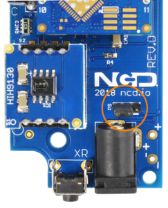
If you are anything like me you’ve already unboxed your Wireless Sensors, possibly behind a locked bathroom door where your children wouldn’t assume they were in need of “fixing” with a wooden hammer. If you have, you are already halfway finished! These devices ship with all the necessary settings to function out of the box. If you plan to use an external power supply all you need to do is plug it in and you are all set, if you are using the included batteries for power, you’ll have to remove the enclosure cover, switch the jumper in the picture so it sits on the two pins farthest away from “PS”, and replace the cover. You are now transmitting telemetry. Of course if you want to actually see what your wireless sensors are transmitting you will also need an XBee router, this should plug directly into your computer using the supplied USB cable. By default these sensors will transmit their data every 10 minutes, you can configure this delay in a few ways, which we will cover in another article.
Setting up Node-RED
Now that you have sensors running, we need a way to do something useful with that data. In the past your options tended to be either A) Hire a developer, or B) Use some proprietary software that probably costs additional money on top of the hardware you’ve already purchased. Our dislike of these options is largely what led us to start building for Node-RED. If you’ve never used it before, I have great news! It’s free, open source, and simple. It works on Windows, Linux and Mac, and is constantly being developed and improved. Seeing no need to reinvent the wheel, I’ll point you to the excellent documentation already available for Installing Node-RED. Once that’s done, you’ll need to enter your command line, or Power Shell for Windows users, navigate to the directory Node-RED is installed in, and type “npm i ncd-red-wireless node-red-dashboard“. This will install the nodes required to receive data from your wireless sensors and complete this tutorial, and you can start Node-RED once this is done.
Setting up the nodes
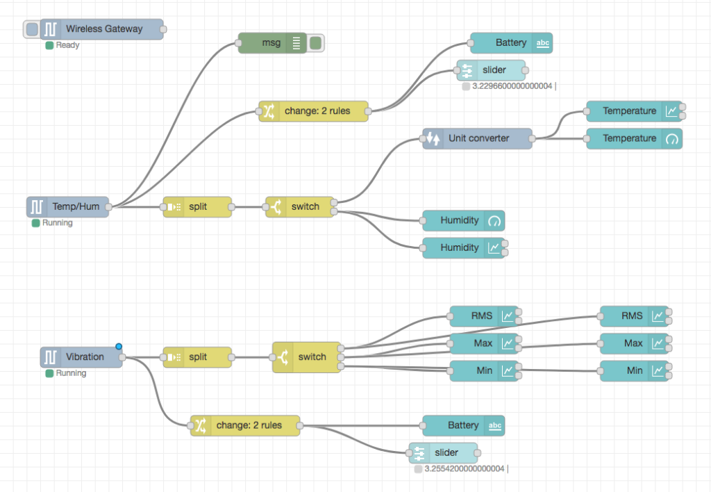
Now, build the flow in the image above to proceed with the tutorial… Just kidding! And don’t worry… this isn’t as bad as it looks. The packages you installed provide a few different pieces of functionality, as detailed here, but you can learn more about each by adding one of the nodes it provides to a flow and viewing its info tab. Assuming at this point you’ve started up Node-RED, you should be able to open a browser and navigate to http://localhost:1880, this will open up the flow builder that is the heart of the Node-RED experience. At this point you’ll be viewing a large blank flow with a long list of nodes on the left hand side, this sidebar is called the palette. At the top of the palette is a search box, if you type “ncd”, the nodes available will be filtered down to those we provided through the ncd-red-wireless package. Go ahead and drag a Wireless Gateway node over to your flow canvas to get started.
ncd-red-wireless
Provides the nodes that manage the serial connection, parse incoming sensor data, filter it by specific parameters, and allow you to configure the wireless sensors.
node-red-dashboard
Provides the ability to create a UI using the flow builder, provides charts, graphs, and a number of other visual elements we can use to display data, along with nodes to trigger a flow using user input. We will use some of these nodes to display the telemetry from your wireless sensors.
Finding your wireless sensors
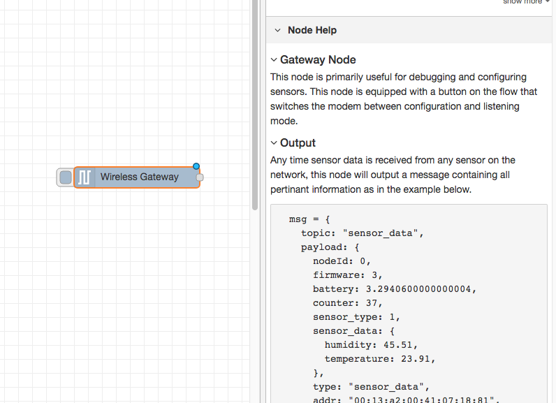
Once you’ve added the node you’ll be able to view the info tab, which contains information about the node’s functionality, this tab is well populated for most node-red packages I have used, and contains valuable information, many times you will not need to view any other documentation outside of the info tab, so keep it in mind while you are building your flows if you have a question about how a node works. The next thing we need to do is configure the node, when you first add it you’ll notice that there is a small triangle on the top right corner next to a blue dot, the triangle indicates that the node needs additional configuration, the blue dot indicates that the node has not yet been deployed as part of the flow.
Double click on the node to open up the configuration options. Click on the pencil icon next to the Serial Device field to configure your USB router, this will open a second configuration panel that only has a few options, click on the magnifying glass next to the Serial Port field and select the port that corresponds with your router, then click the “Add” button on top. The Serial Device field will now be populated based on that selection, and you can click “Done”, you now have direct access to your wireless sensors! To view the data coming in, go back to your palette and type “debug” into the search field at the top, grab one of these nodes and drag it to the right of your Wireless Gateway, double click on it and change “msg.” to “complete msg object”, click done, and draw a line between the two nodes, and click “Deploy” on the top right of the window..
Working with the data
You are now collecting data from your wireless sensors, and outputting it to the “debug” tab, this is located in the right sidebar next to the info tab. Clicking the reset button on one of your sensors should force an update and you can see the data come in. In Node-RED data is passed between nodes in a JSON packet, if you are unfamiliar with JSON, it is simply an object notation that was originally used for Javascript, and has since been adopted as a standard across many APIs for it’s simplicity and flexibility. When the msg object comes in to the debug tab you can expand it to view the full list of information that comes with it. This is extremely helpful if you need to quickly see which sensors are checking in, or if you simply want to push all incoming data up to a cloud service and handle the aggregation and data manipulation there. The other thing this node provides is a simple way to switch your router to the network ID that devices in configuration mode report on, simply click the button on the left of the node and the device will switch to the configuration network, click it again to return it to listening mode. Once we get the Wireless Device nodes set up, they can be set to automatically configure a sensor when it enters configuration mode, so it’s always handy to keep one of these Gateway nodes present on the flow for quickly configuring a device.
Adding the wireless sensors
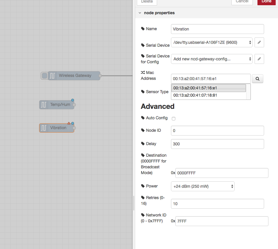
For the purposes of this tutorial, we want to separate wireless sensor data locally so that we can display it, we could use a switch node to split out the messages from the gateway based on the mac address or sensor type, but as I mentioned, the Wireless Nodes actually contain additional functionality for configuring the sensors, so we’ll start with them to give you a more complete picture of how these systems can work. If you haven’t already seen packets coming in from both of your sensors, go ahead and hit the reset button on the one that hasn’t reported. When a sensor checks in through any Serial Device configuration node, the mac address and type of sensor is cached in a pool so we can quickly find it during this next step. Grab a Wireless Node from the palette and drag it onto the flow, double click on it to get it configured, and select the serial device from the drop down that you used for the Wireless Gateway, now click the magnifying glass next to “Mac Address” and select one of the available options. You’ll notice this automatically sets the sensor type for you, you can also give it a name to make it easier to identify. As noted in the info tab, the Serial Device for Config field is optional, and we won’t worry about it right now. The node you have just added effectively works as a filter on incoming sensor data, only passing through data for the mac address, or sensor type if no mac address is present. Repeat this process for your other sensor, you should now have a Temperature/Humidity node and a Vibration node.
Displaying up the Temperature/Humidity
These nodes for the wireless sensors output a msg object with all of the same information as the Wireless Gateway node, just in a slightly different format, the Sensor Data itself is sent in the msg.payload, which is what most nodes use to interact with the msg itself.
Grab a “split” node from the palette, and place it to the right of the Temp/Hum node, double click and check the box under Object that says “Copy key to”, this will split the msg into multiple objects, one for each property in the payload, and set the topics for those new msgs to the property names.
Now add a “switch” node, this will allow us to send each msg to a specific part of the flow, one to handle temperature, and one humidity. In the first field change “payload” to “topic”, next to the “==”, type “temperature” then click the “+add” button at the bottom left, in the new field type “humidity”. As you can see each of these has a unique number to the right, this number indicates which output the msg will be sent to when it matches the condition.
Next let’s add a “gauge” from the palette, set the Label to “Temperature”, and the Value format to “{{value | number:2}}”, and the Units to “Celsius” you can alter the range to the minimum and maximum expected temperature, I’m using 0 and 50.
Another really cool feature of the flow builder is copy+paste, click on the gauge you just added and click ctrl+c (cmd+c on mac), then cntl+v, now you have a second gauge, double click on it to change the Label to Humidity, the Units to RH, and the range to 20 and 80.
Now draw wires from the Temperature/Humidity node to the split node, from the split node to the switch node, and from the switch node’s first (top) output to the temperature gauge node, and from the switch node’s second output to the humidity gauge.
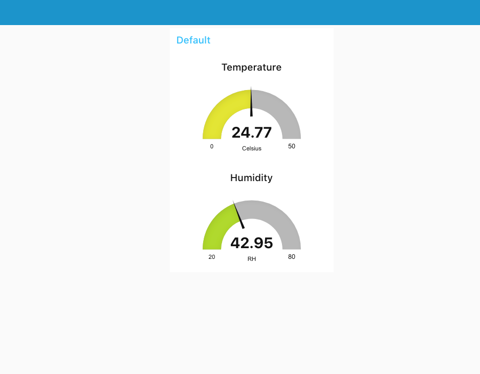
Once that’s done click deploy and let’s check it out! There is a tab on the top right that says “Dashboard”, on the top right of that tab is the little “new window” icon, click on it to view your UI. It is likely that the gauges aren’t displaying any information, because no sensor data has been reported since you deployed the flow, click the reset button on your temperature/humidity sensor to force it to check in and your gauges should jump up. You should now have real time data displaying!
Displaying up the Vibration Data
Setting up the Vibration sensor is very similar to the Temperature/Humidity sensor, we actually start the same way, you can copy and paste the split node you used in the last step and position it next to the Vibration node, we also need a switch node, but it needs to be set up a little bit differently. We’ll still change “payload” to “topic”, but we’re going to use RegExP, or Regular Expressions to actually do the property comparison. Regular Expressions are sequences of characters that define a search pattern, they can be used to test strings, and extract portions of them. In this case we’ll be using a very simple “starts with” regex. Click on the “==” and select “matches regex”, in the field next to it type “rms_.*”, this means “match a string that contains rms_ followed by any character (.) as many characters as are available (*). Add a new row and follow the last step, replacing “rms” with “max”, and then one more time with “min”. This will split our incoming payloads into 3 sections to be routed to ui, each containing the appropriate values for all 3 axes.
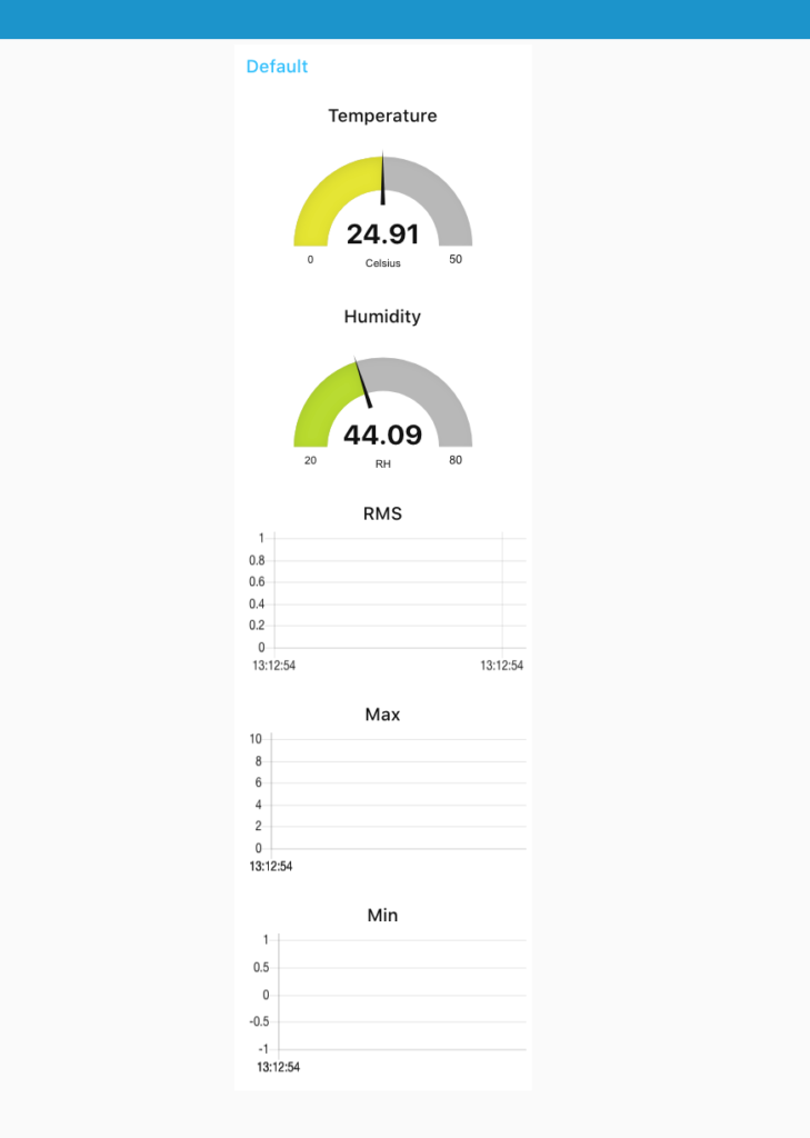
We’ll use chart nodes for this sensor, so grab one from the palette and bring it over. Set the Label to RMS, and that’s it… you now have a chart. Go ahead and copy it a couple of times, setting the subsequent labels to Min and Max, and draw the wires from the switch, output 1 -> RMS, 2 -> Min, and 3 -> Max.
Go ahead and deploy and click reset on the vibration sensor to start sending data. Take a look at your new UI, the charts are obviously a bit sparse with only 1 X-axis point, In this case resetting the sensor won’t help unless you are moving it while it resets, if it is sitting flat on your desk it will just send out the initial values (0) when it starts up, making for a very boring chart.
You can set the check in interval lower using the Vibration node pretty easily however, go to your flow and double click on it, under the “Advanced” heading check the “Auto Config” box and change the delay to something smaller, say, 10 (this is in seconds). The rest of the settings are already set at the defaults for the sensor, go ahead and deploy the flow. Now click the button on the Wireless Gateway node, this will put in on the network to configure the devices. On the vibration sensor click the reset button, once you’ve released it hold down the config button for 5 or 6 seconds, when you let up you should see the status of the Vibration node cycling through configuration steps. When it says complete, click the reset button again and you will start receiving data more frequently to fill the chart.
Wrapping up
As you can see, the power of Node-RED lies in its simplicity, while there are several steps to get to this point, they are all easy to replicate, and require literally no programming to take your wireless sensors from the box to the dashboard. I won’t delve into all of the options available for the dashboard here, there is some great information on the GitHub page, and most of what I’ve used here I figured out through trial and error, I encourage you to do the same. There is a tremendous following developing for, and using, Node-RED in production environments around the world, and we are very excited to be able to bring our product line into this growing community. If you have any questions about Node-RED as it relates to our products, please feel free to jump on our community. We have a category we set up just for this amazing framework you can find here. Below is an export of the complete dashboard setup I built for these wireless sensors, complete with a history tab. Feel free to grab and use it, you will need to set the Serial Devices on the appropriate nodes that will be marked with a triangle. To import this flow, copy the JSON below to your clipboard, click on the hamburger on the top right of your flow builder, hover over import and click “clipboard”, then just paste it in and click the import button. Have fun!
TLDR; Import this Flow
[{"id":"bf698a47.fa5548","type":"ncd-wireless-node","z":"13754c0b.dca3a4","name":"Temp/Hum","connection":"","config_comm":"","addr":"","sensor_type":"1","auto_config":true,"node_id":0,"delay":"5","destination":"0000FFFF","power":"1","retries":10,"pan_id":"7FFF","change_enabled":false,"change_pr":"0","change_interval":"0","cm_calibration":"0","bp_altitude":"0","bp_pressure":"0","bp_temp_prec":"0","bp_press_prec":"0","amgt_accel":"0","amgt_mag":"0","amgt_gyro":"0","x":120,"y":320,"wires":[["7389919e.396ca","c98d662.aee9398"]]},{"id":"7fa37cc0.553844","type":"ui_gauge","z":"13754c0b.dca3a4","name":"","group":"ebd2860b.d0fc78","order":5,"width":"12","height":"6","gtype":"gage","title":"Temperature","label":"Fahrenheit","format":"{{value|number:2}}","min":"32","max":"120","colors":["#000cb5","#00e61a","#ca0002"],"seg1":"","seg2":"","x":950,"y":220,"wires":[]},{"id":"7389919e.396ca","type":"split","z":"13754c0b.dca3a4","name":"","splt":"\\n","spltType":"str","arraySplt":1,"arraySpltType":"len","stream":false,"addname":"topic","x":310,"y":320,"wires":[["7526501a.d1dc2"]]},{"id":"7526501a.d1dc2","type":"switch","z":"13754c0b.dca3a4","name":"","property":"topic","propertyType":"msg","rules":[{"t":"eq","v":"temperature","vt":"str"},{"t":"eq","v":"humidity","vt":"str"}],"checkall":"true","repair":false,"outputs":2,"x":460,"y":320,"wires":[["4a6a97fc.739288"],["92a172e6.aea14","5660668.d40b798"]]},{"id":"92a172e6.aea14","type":"ui_gauge","z":"13754c0b.dca3a4","name":"","group":"ebd2860b.d0fc78","order":6,"width":"12","height":"6","gtype":"gage","title":"Humidity","label":"RH","format":"{{value|number:2}}","min":"20","max":"80","colors":["#00b500","#c9e625","#ca1c02"],"seg1":"","seg2":"","x":700,"y":340,"wires":[]},{"id":"5fafbbea.184774","type":"ui_chart","z":"13754c0b.dca3a4","name":"","group":"3d4868ac.9084c8","order":0,"width":"12","height":"6","label":"Temperature","chartType":"line","legend":"false","xformat":"HH:mm:ss","interpolate":"linear","nodata":"","dot":false,"ymin":"","ymax":"","removeOlder":1,"removeOlderPoints":"","removeOlderUnit":"86400","cutout":0,"useOneColor":false,"colors":["#1f77b4","#aec7e8","#ff7f0e","#2ca02c","#98df8a","#d62728","#ff9896","#9467bd","#c5b0d5"],"useOldStyle":false,"x":950,"y":180,"wires":[[],[]]},{"id":"5660668.d40b798","type":"ui_chart","z":"13754c0b.dca3a4","name":"","group":"3d4868ac.9084c8","order":0,"width":"12","height":"6","label":"Humidity","chartType":"line","legend":"false","xformat":"HH:mm:ss","interpolate":"linear","nodata":"","dot":false,"ymin":"","ymax":"","removeOlder":1,"removeOlderPoints":"","removeOlderUnit":"86400","cutout":0,"useOneColor":false,"colors":["#1f77b4","#aec7e8","#ff7f0e","#2ca02c","#98df8a","#d62728","#ff9896","#9467bd","#c5b0d5"],"useOldStyle":false,"x":700,"y":380,"wires":[[],[]]},{"id":"400cba0d.021bd4","type":"ncd-wireless-node","z":"13754c0b.dca3a4","name":"Vibration","connection":"","config_comm":"","addr":"","sensor_type":"13","auto_config":true,"node_id":0,"delay":"5","destination":"0000FFFF","power":"1","retries":10,"pan_id":"7FFF","change_enabled":false,"change_pr":"0","change_interval":"0","cm_calibration":"0","bp_altitude":"0","bp_pressure":"0","bp_temp_prec":"0","bp_press_prec":"0","amgt_accel":"0","amgt_mag":"0","amgt_gyro":"0","x":140,"y":540,"wires":[["af59356d.0f23f8","9a2a7cbf.76161"]]},{"id":"3800bb26.f824a4","type":"ui_chart","z":"13754c0b.dca3a4","name":"","group":"60afd6aa.b52828","order":1,"width":"12","height":"6","label":"RMS","chartType":"line","legend":"true","xformat":"HH:mm:ss","interpolate":"bezier","nodata":"","dot":false,"ymin":"","ymax":"","removeOlder":"10","removeOlderPoints":"","removeOlderUnit":"60","cutout":0,"useOneColor":false,"colors":["#1f77b4","#aec7e8","#ff7f0e","#2ca02c","#98df8a","#d62728","#ff9896","#9467bd","#c5b0d5"],"useOldStyle":false,"x":730,"y":480,"wires":[[],[]]},{"id":"af59356d.0f23f8","type":"split","z":"13754c0b.dca3a4","name":"","splt":"\\n","spltType":"str","arraySplt":1,"arraySpltType":"len","stream":false,"addname":"topic","x":310,"y":540,"wires":[["e24a52cf.d53e2"]]},{"id":"e24a52cf.d53e2","type":"switch","z":"13754c0b.dca3a4","name":"","property":"topic","propertyType":"msg","rules":[{"t":"regex","v":"rms_.*","vt":"str","case":false},{"t":"regex","v":"max_.*","vt":"str","case":false},{"t":"regex","v":"min_.*","vt":"str","case":false}],"checkall":"true","repair":false,"outputs":3,"x":470,"y":540,"wires":[["3800bb26.f824a4","8aecc887.85b3a8"],["d70ac318.f5cce","722bb814.a1f818"],["8e302384.dab27","8dbd1766.9b52a8"]]},{"id":"d70ac318.f5cce","type":"ui_chart","z":"13754c0b.dca3a4","name":"","group":"60afd6aa.b52828","order":2,"width":"6","height":"6","label":"Max","chartType":"line","legend":"true","xformat":"HH:mm:ss","interpolate":"bezier","nodata":"","dot":false,"ymin":"","ymax":"","removeOlder":"10","removeOlderPoints":"","removeOlderUnit":"60","cutout":0,"useOneColor":false,"colors":["#1f77b4","#aec7e8","#ff7f0e","#2ca02c","#98df8a","#d62728","#ff9896","#9467bd","#c5b0d5"],"useOldStyle":false,"x":730,"y":520,"wires":[[],[]]},{"id":"8e302384.dab27","type":"ui_chart","z":"13754c0b.dca3a4","name":"","group":"60afd6aa.b52828","order":3,"width":"6","height":"6","label":"Min","chartType":"line","legend":"true","xformat":"HH:mm:ss","interpolate":"bezier","nodata":"","dot":false,"ymin":"","ymax":"","removeOlder":"10","removeOlderPoints":"","removeOlderUnit":"60","cutout":0,"useOneColor":false,"colors":["#1f77b4","#aec7e8","#ff7f0e","#2ca02c","#98df8a","#d62728","#ff9896","#9467bd","#c5b0d5"],"useOldStyle":false,"x":730,"y":560,"wires":[[],[]]},{"id":"8aecc887.85b3a8","type":"ui_chart","z":"13754c0b.dca3a4","name":"","group":"8b6cb092.e5788","order":0,"width":"12","height":"6","label":"RMS","chartType":"line","legend":"true","xformat":"HH:mm:ss","interpolate":"bezier","nodata":"","dot":false,"ymin":"","ymax":"","removeOlder":"1","removeOlderPoints":"","removeOlderUnit":"86400","cutout":0,"useOneColor":false,"colors":["#1f77b4","#aec7e8","#ff7f0e","#2ca02c","#98df8a","#d62728","#ff9896","#9467bd","#c5b0d5"],"useOldStyle":false,"x":950,"y":480,"wires":[[],[]]},{"id":"722bb814.a1f818","type":"ui_chart","z":"13754c0b.dca3a4","name":"","group":"8b6cb092.e5788","order":0,"width":"6","height":"6","label":"Max","chartType":"line","legend":"true","xformat":"HH:mm:ss","interpolate":"bezier","nodata":"","dot":false,"ymin":"","ymax":"","removeOlder":"1","removeOlderPoints":"","removeOlderUnit":"86400","cutout":0,"useOneColor":false,"colors":["#1f77b4","#aec7e8","#ff7f0e","#2ca02c","#98df8a","#d62728","#ff9896","#9467bd","#c5b0d5"],"useOldStyle":false,"x":950,"y":520,"wires":[[],[]]},{"id":"8dbd1766.9b52a8","type":"ui_chart","z":"13754c0b.dca3a4","name":"","group":"8b6cb092.e5788","order":0,"width":"6","height":"6","label":"Min","chartType":"line","legend":"true","xformat":"HH:mm:ss","interpolate":"bezier","nodata":"","dot":false,"ymin":"","ymax":"","removeOlder":"1","removeOlderPoints":"","removeOlderUnit":"86400","cutout":0,"useOneColor":false,"colors":["#1f77b4","#aec7e8","#ff7f0e","#2ca02c","#98df8a","#d62728","#ff9896","#9467bd","#c5b0d5"],"useOldStyle":false,"x":950,"y":560,"wires":[[],[]]},{"id":"67f6efbd.53daa","type":"ui_slider","z":"13754c0b.dca3a4","name":"","label":"","group":"ebd2860b.d0fc78","order":8,"width":0,"height":0,"passthru":false,"topic":"","min":0,"max":"3.3","step":".1","x":740,"y":120,"wires":[[]]},{"id":"c98d662.aee9398","type":"change","z":"13754c0b.dca3a4","name":"","rules":[{"t":"set","p":"payload","pt":"msg","to":"data.battery","tot":"msg"},{"t":"set","p":"enabled","pt":"msg","to":"false","tot":"bool"}],"action":"","property":"","from":"","to":"","reg":false,"x":480,"y":180,"wires":[["67f6efbd.53daa","94647165.b8107"]]},{"id":"94647165.b8107","type":"ui_text","z":"13754c0b.dca3a4","group":"ebd2860b.d0fc78","order":7,"width":0,"height":0,"name":"","label":"Battery","format":"{{msg.payload|number:3}}V","layout":"row-center","x":770,"y":80,"wires":[]},{"id":"2874f1a4.b8c8ce","type":"ui_slider","z":"13754c0b.dca3a4","name":"","label":"","group":"60afd6aa.b52828","order":5,"width":0,"height":0,"passthru":false,"topic":"","min":0,"max":"3.3","step":".1","x":670,"y":680,"wires":[[]]},{"id":"9a2a7cbf.76161","type":"change","z":"13754c0b.dca3a4","name":"","rules":[{"t":"set","p":"payload","pt":"msg","to":"data.battery","tot":"msg"},{"t":"set","p":"enabled","pt":"msg","to":"false","tot":"bool"}],"action":"","property":"","from":"","to":"","reg":false,"x":380,"y":640,"wires":[["2874f1a4.b8c8ce","4028f5a3.b9687c"]]},{"id":"4028f5a3.b9687c","type":"ui_text","z":"13754c0b.dca3a4","group":"60afd6aa.b52828","order":4,"width":0,"height":0,"name":"","label":"Battery","format":"{{msg.payload|number:3}}V","layout":"row-center","x":700,"y":640,"wires":[]},{"id":"786bff29.83c1f","type":"ncd-gateway-node","z":"13754c0b.dca3a4","name":"","connection":"","x":170,"y":160,"wires":[["e2d8807d.240c6"]]},{"id":"e2d8807d.240c6","type":"debug","z":"13754c0b.dca3a4","name":"","active":true,"tosidebar":true,"console":false,"tostatus":false,"complete":"true","x":400,"y":100,"wires":[]},{"id":"4a6a97fc.739288","type":"function","z":"13754c0b.dca3a4","name":"","func":"msg.payload = (msg.payload * 1.8) + 32;\nreturn msg;","outputs":1,"noerr":0,"x":710,"y":240,"wires":[["5fafbbea.184774","7fa37cc0.553844"]]},{"id":"ebd2860b.d0fc78","type":"ui_group","z":"","name":"Environment","tab":"4c7c29de.f9ea38","disp":true,"width":"12","collapse":false},{"id":"3d4868ac.9084c8","type":"ui_group","z":"","name":"Environment","tab":"38410f18.307bb","disp":true,"width":"12","collapse":false},{"id":"60afd6aa.b52828","type":"ui_group","z":"","name":"Vibration","tab":"4c7c29de.f9ea38","disp":true,"width":"12","collapse":false},{"id":"8b6cb092.e5788","type":"ui_group","z":"","name":"Vibration","tab":"38410f18.307bb","disp":true,"width":"12","collapse":false},{"id":"4c7c29de.f9ea38","type":"ui_tab","z":"","name":"Current","icon":"dashboard"},{"id":"38410f18.307bb","type":"ui_tab","z":"","name":"History","icon":"dashboard"}]