Enterprise Wireless Vibration Sensor Product Manual

Overview

Features

  • Industrial Grade 3-axis Vibration Sensor with RMS, MAX and MIN acceleration in g
  • Time Domain data transmission for Time/Frequency domain Analysis
  • Vibration Range ±16g
  • Noise Removal using Multiple Low pass filters and Over sampling
  • Configurable Bandwidth: 58 Hz to 12.8 kHz
  • Configurable Sampling Rate 400 Hz to 25.6 kHz
  • Built-in Offset and Gravity vector removal filters
  • Built-in 6-point calibration for 0-g Offset and Sensitivity adjustment
  • Temperature output with an accuracy of ±1°C
  • Operating Temperature Range -40 to +85 °C
  • 1-Mile Range with 2.4GHz or 2 Mile Range with 900MHz On-Board Antenna
  • Superior LOS Range of up to 28 miles with 900MHz High-Gain Antennas
  • Interface to Raspberry Pi, Microsoft Azure, Arduino and More
  • Example Software for Visual Studio and LabVIEW
  • Wireless Mesh Networking using DigiMesh®
  • Up to 256 Sensor Nodes per Network
  • Open Communication Protocol for custom interfacing applications
  • Small Form Factor (3×3 inch)
  • Multiple Modes of Operation (Configuration and Run mode)
  • Wireless Sensor and Radio Configuration feature
  • Default Factory setting Restore option
  • Power Efficient Built-in Sleep mode
  • User Configurable Sleep duration
  • Up to 500,000 Transmissions from 2 AA Batteries
  • Reliable Transmission incorporating packet Retries
  • Secure Transmission using AES-128 Encryption
  • Real time battery status

Applications

  • Wireless Industrial Machine Health Analysis
  • Machine Fault detection
  • Frequency Analysis of Vibration data
  • Building and Structural Monitoring

Description

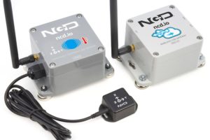
Introducing NCD’s Enterprise Wireless Vibration Sensor, boasting up to a 28 Mile range using a 900MHz wireless mesh networking architecture or 1 Mile using 2.4GHz wireless mesh networking architecture. Incorporating an DC coupled acceleration sensor and a temperature sensor, the frequency response is from 0 Hz to user defined upper cutoff frequency. It samples and processes vibration data at user defined sampling rate and bandwidth, and then transmits this information to user defined receiver(s). The whole process is repeated at user defined intervals.

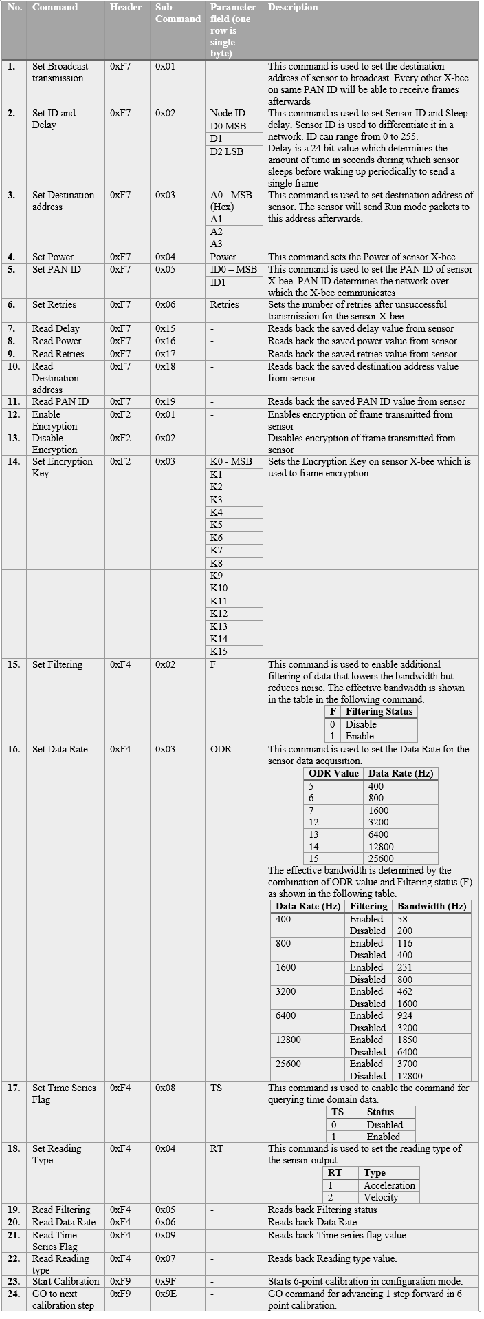
The Enterprise Wireless Vibration Sensor removes the offsets and accounts for sensitivity variation of the internal sensing element. It has an internal memory which stores the 0-g offsets and sensitivities for each axis. Default factory saved values usually provide the required accuracy, however, the sensor incorporates a 6-point calibration routine that can be initiated in the configuration mode by the user to carry out 6-point calibration as described in configuration section. This process overrides the factory default values however, the settings can be restored as discussed in troubleshooting section.

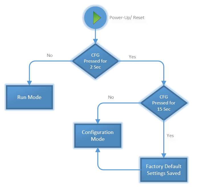
At power up or reset, the sensor calibrates itself so that it can remove 0-g offsets as well as gravity vector from future readings. This process may take up 10 seconds. This process does not require the sensor to be placed on a stationary platform. Hence, it can be mounted on running machines at any angle and a simple reset of the sensor allows it to calibrate itself.

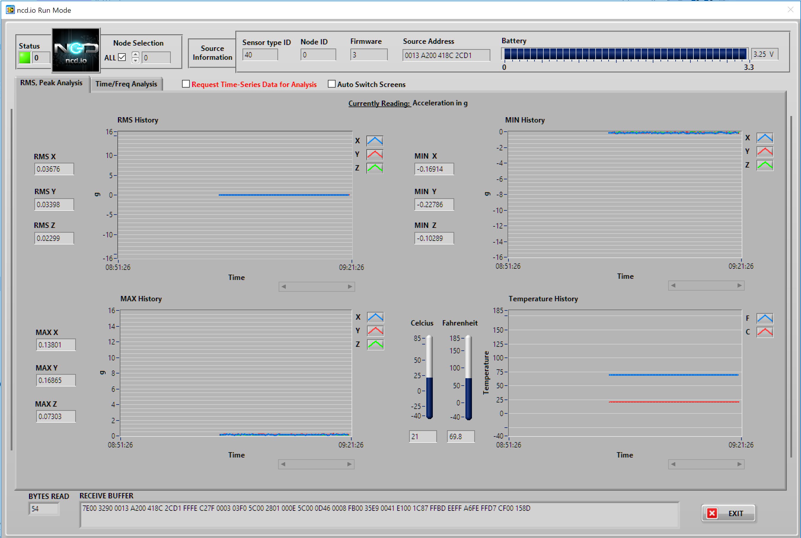
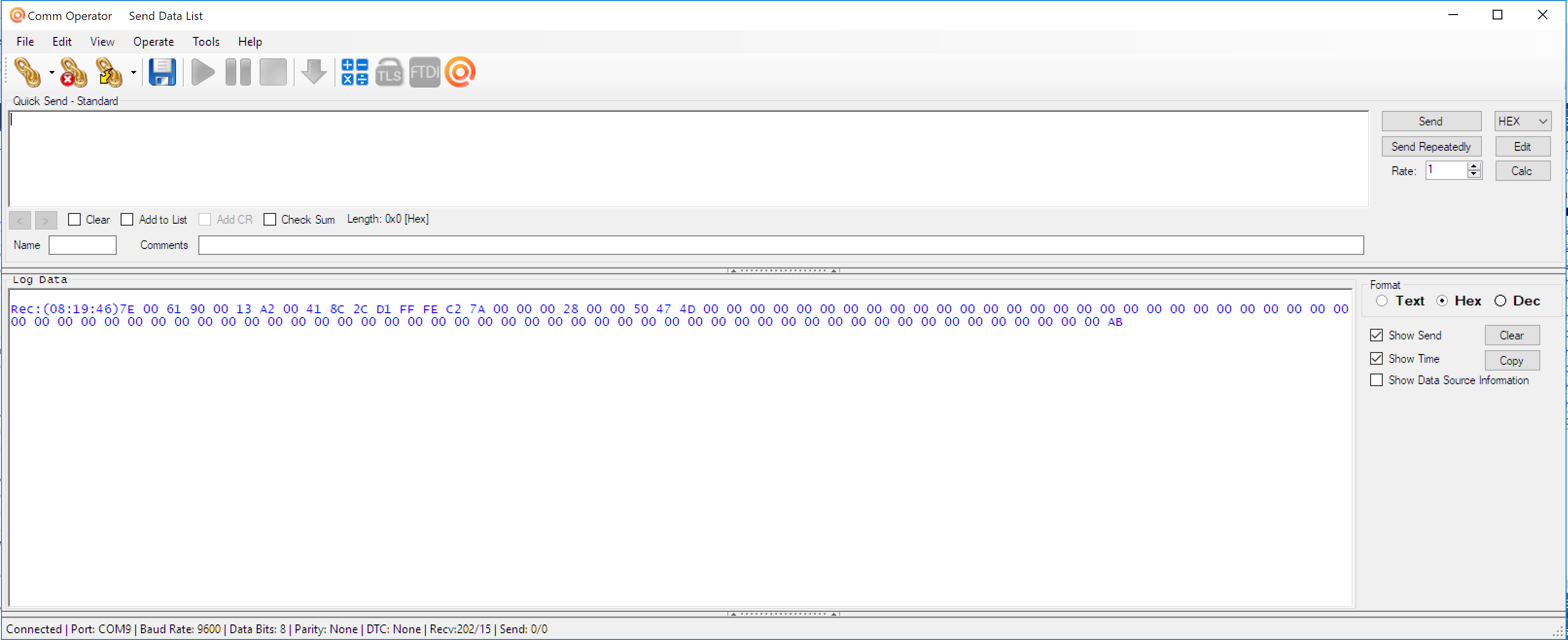
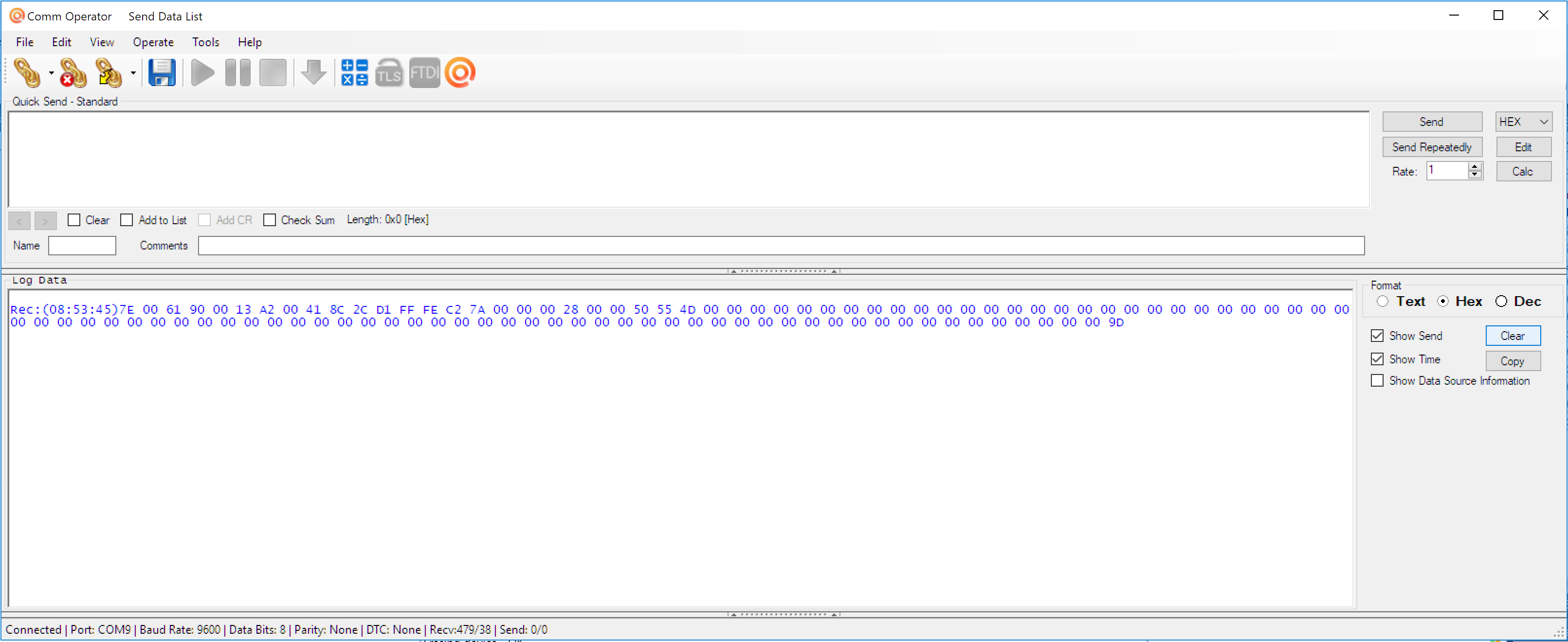
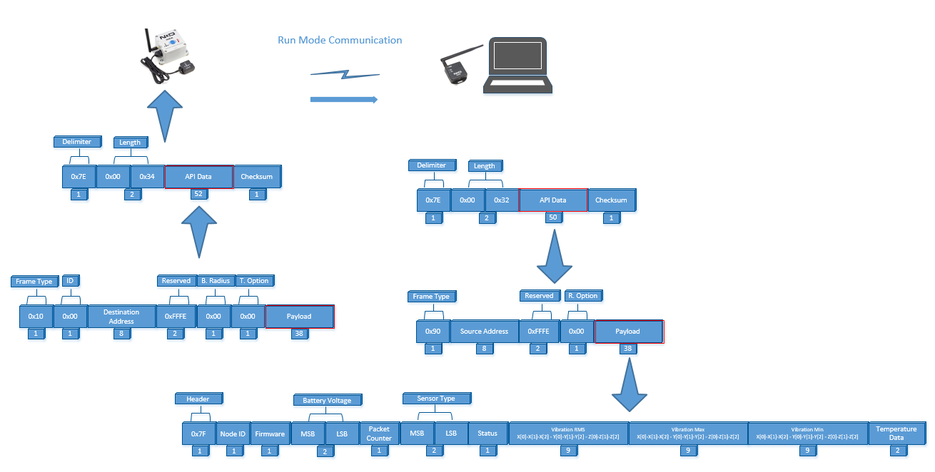
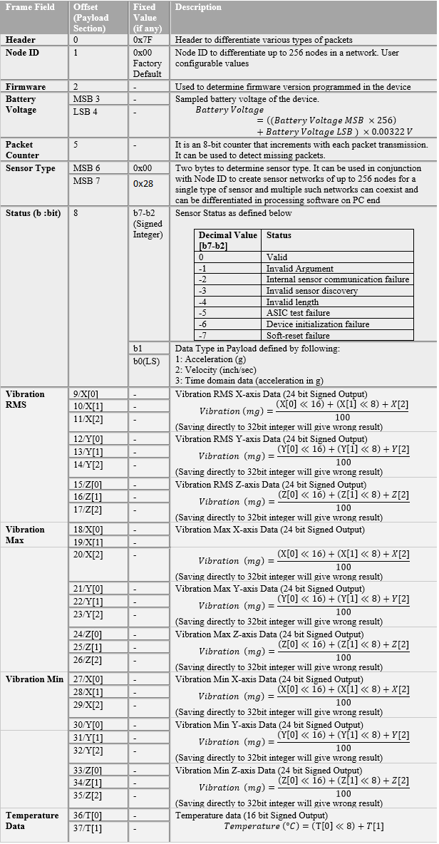
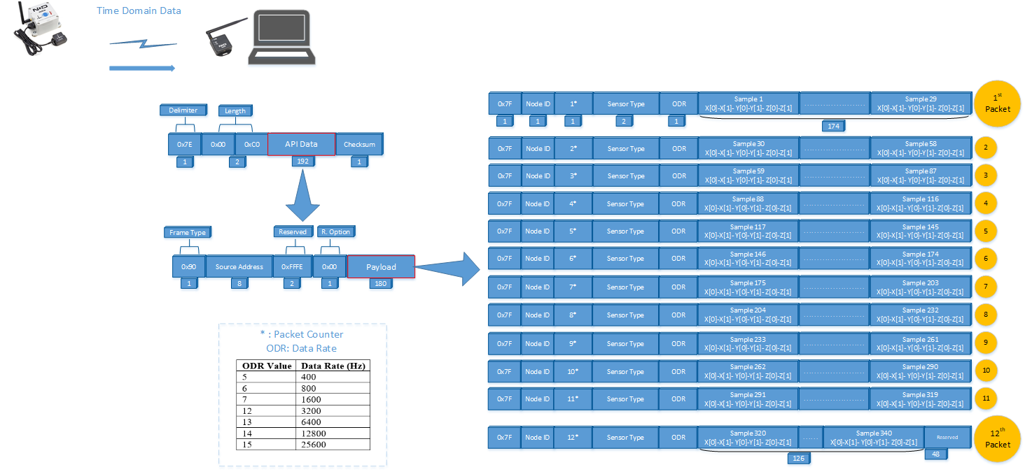
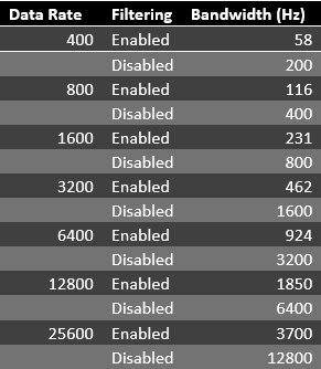
The sensor accumulates 340 samples for each of the 3-axis and processes them to calculate RMS, Maximum and Minimum Vibration in this interval. The sample accumulation period thus varies with the configurable sampling rate. A low sampling rate increases the sample accumulation period, hence care should be exercised since it increases the duration for which the sensor is powered up and thus drains the battery. For example, sample accumulation period for a sampling rate of 400 Hz turns out to be  850msec, whereas, for a sampling rate of 25.6 kHz, it is reduced to13.3msec. The resultant information is then combined with temperature read from a temperature sensor and sent to one or multiple receivers. After data transmission, the sensor goes to sleep for a user defined interval, thus minimizing power consumption.

Powered by just 2 AA batteries and an operational lifetime of 500,000 wireless transmissions, a 5 years battery life can be expected depending on environmental conditions and the data transmission interval. Optionally, this sensor may be externally powered.

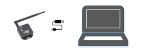
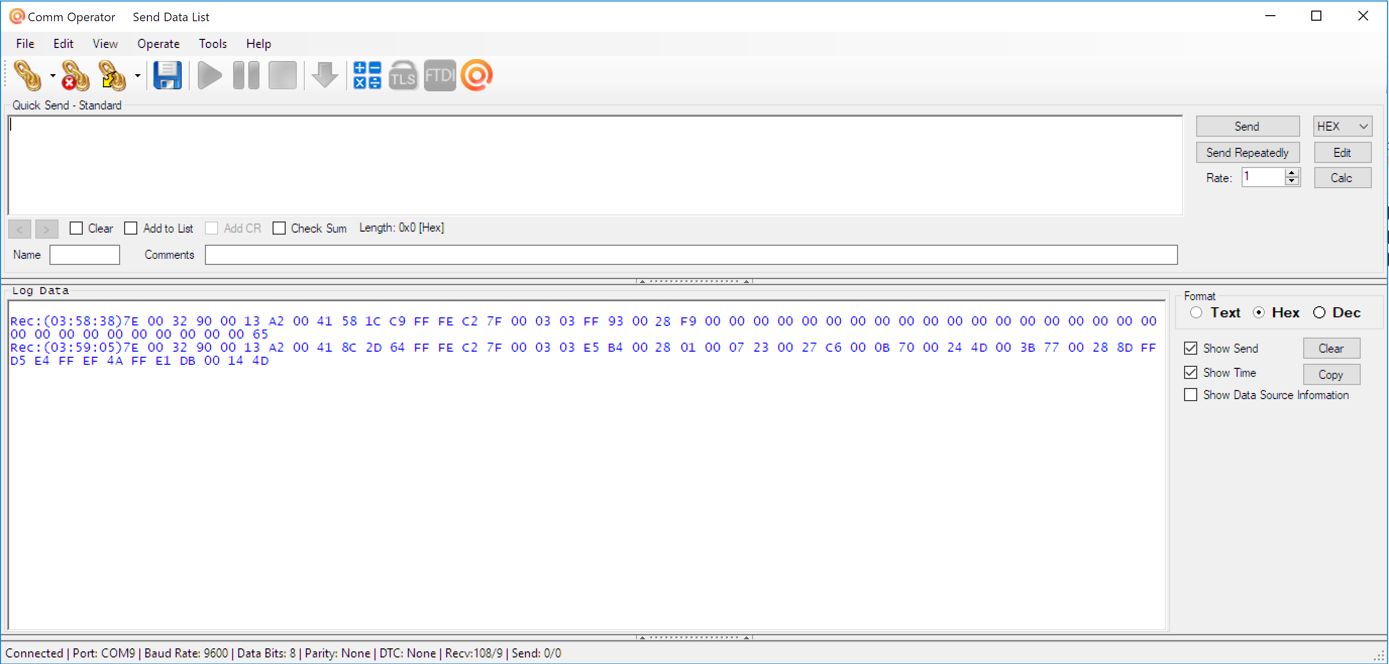
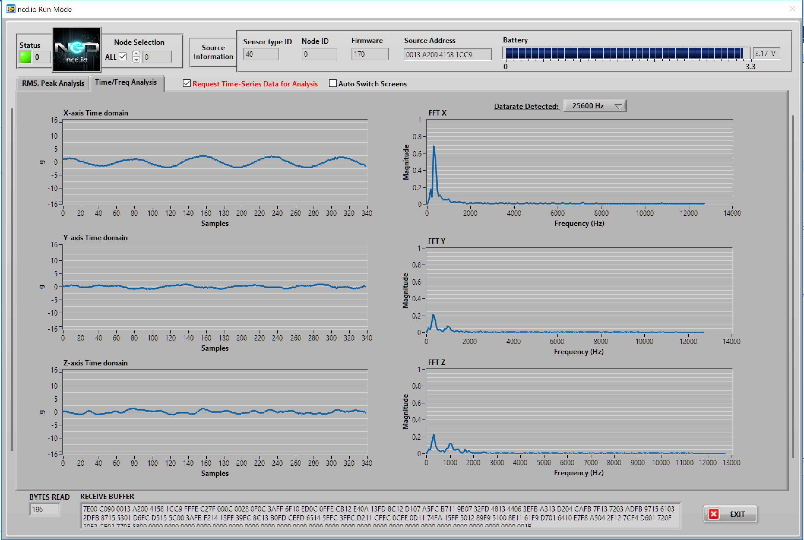
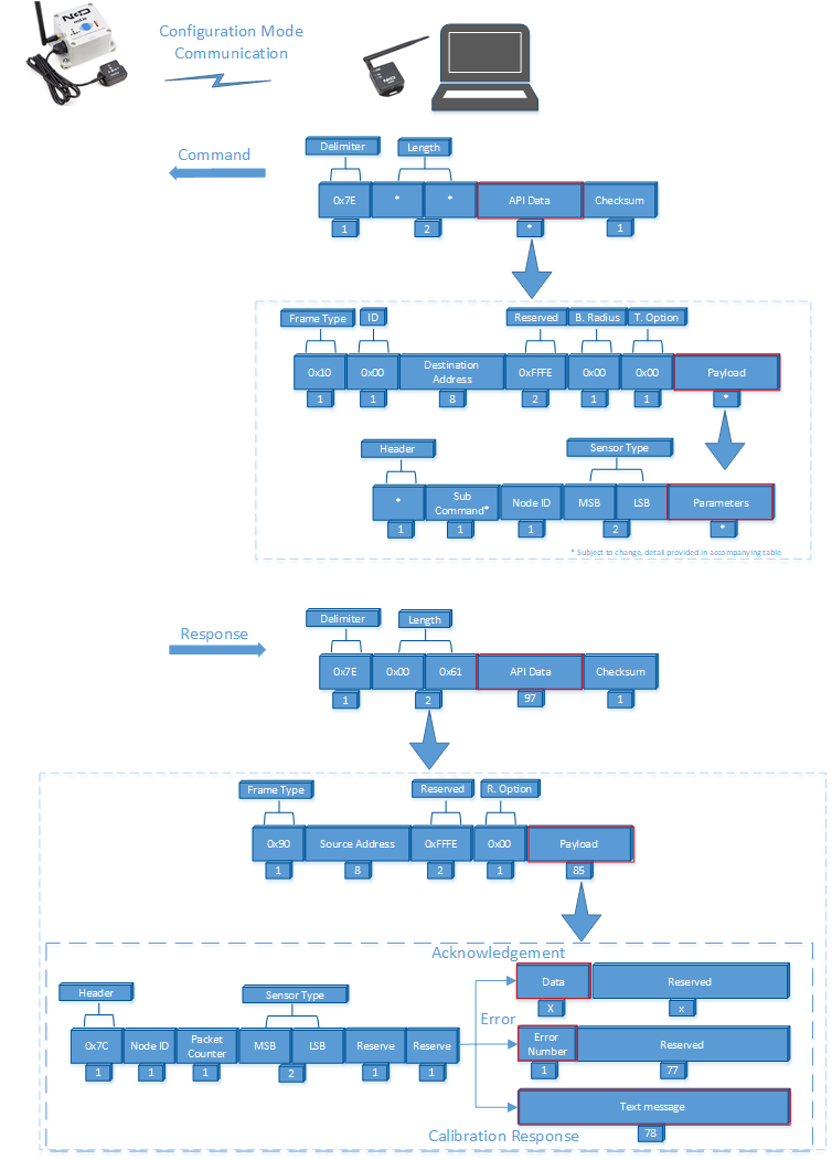
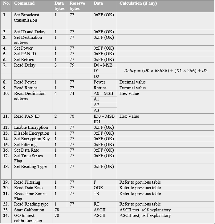
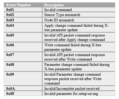
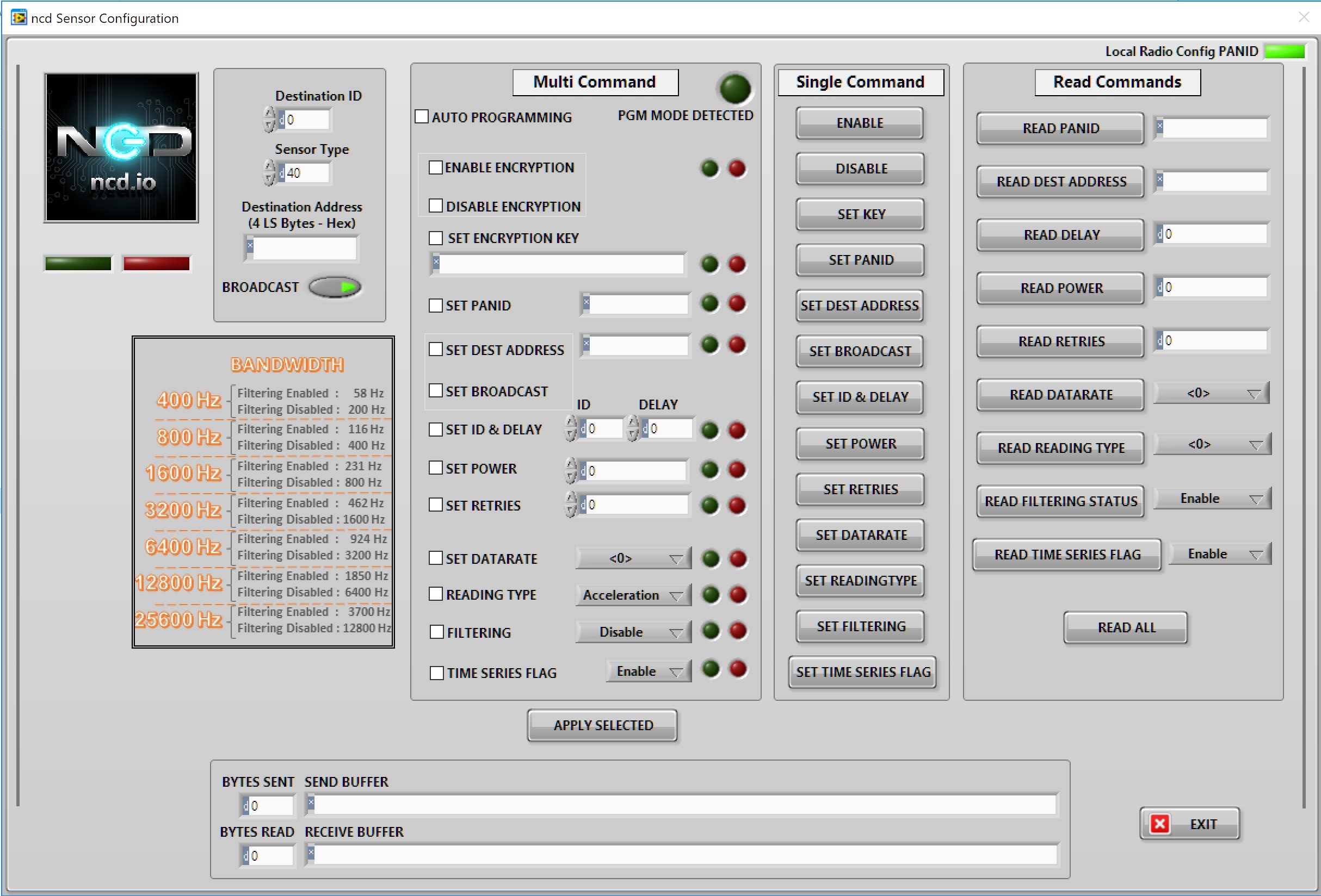
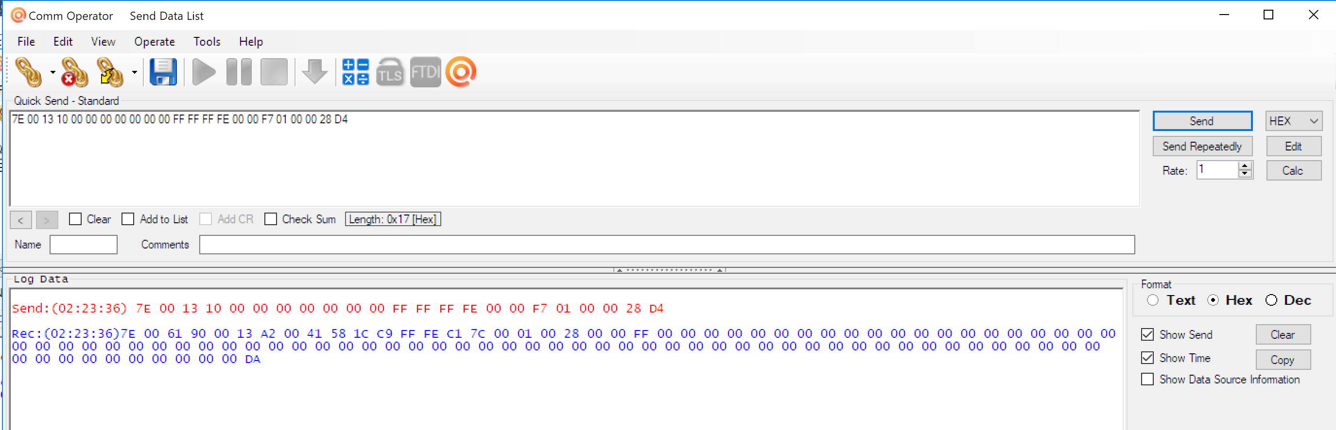
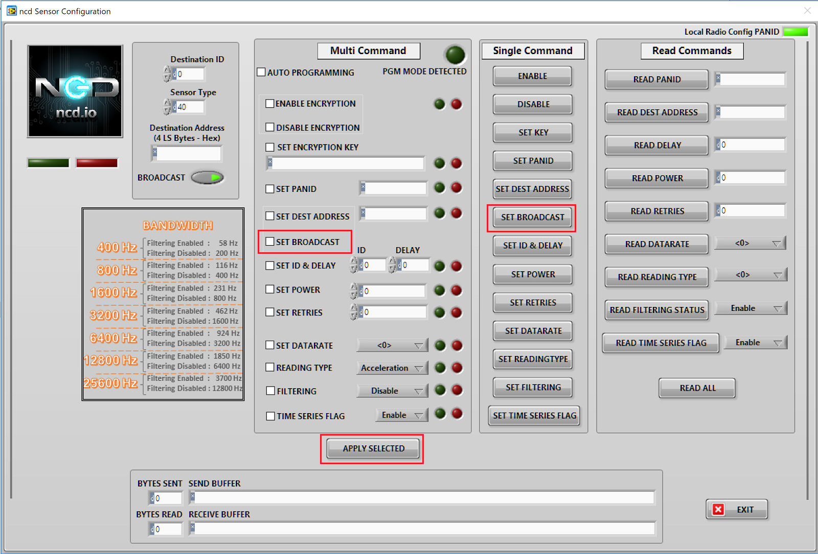
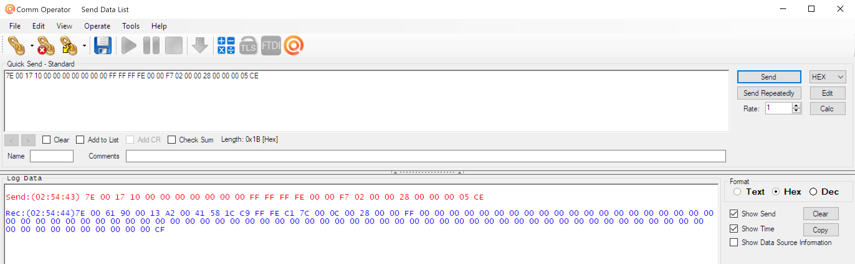
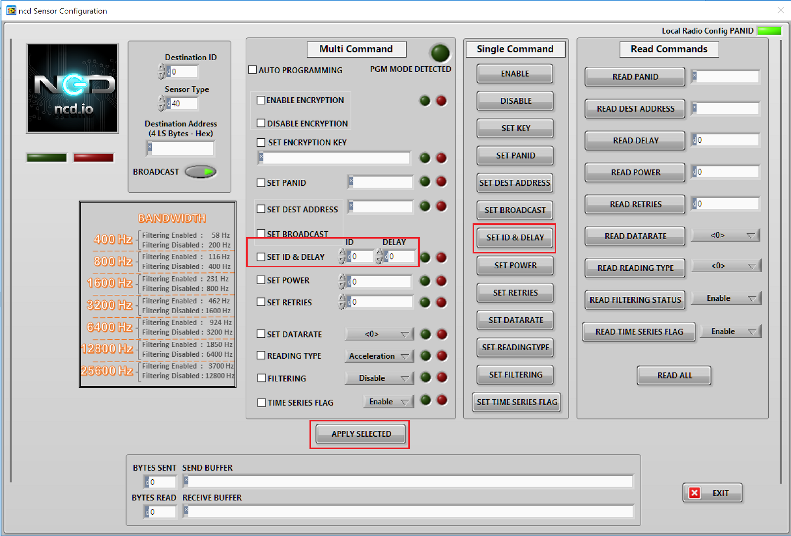
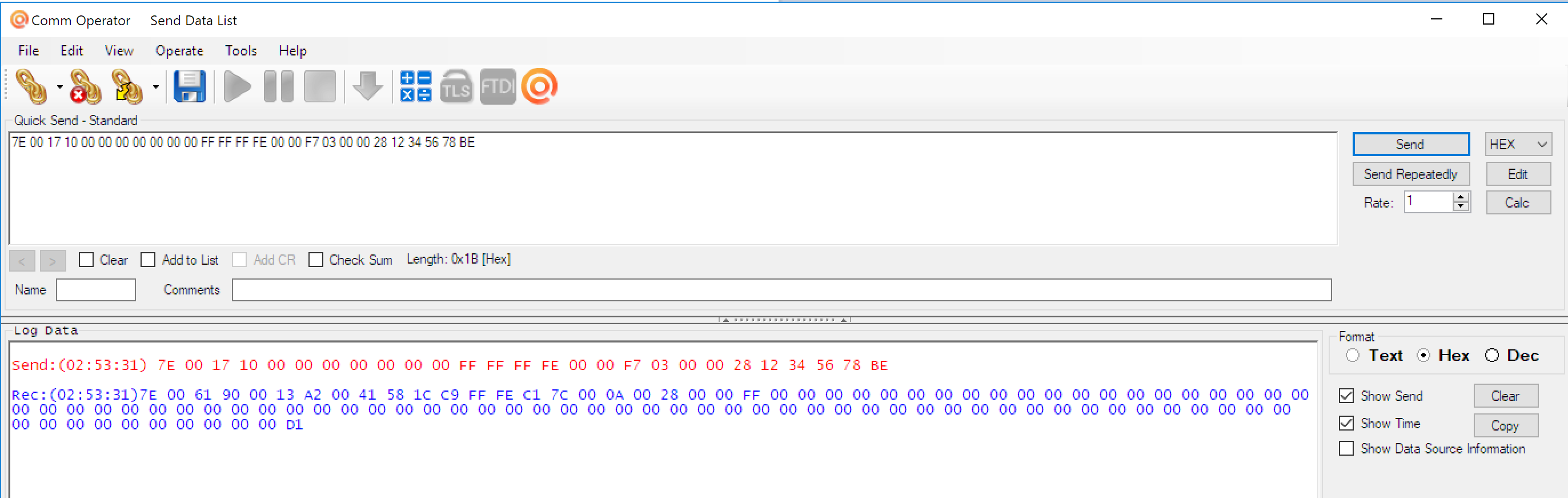
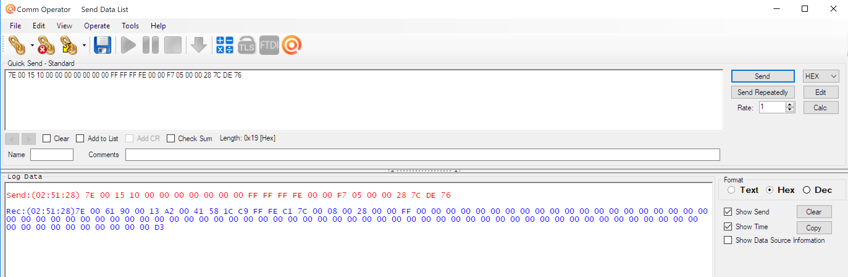
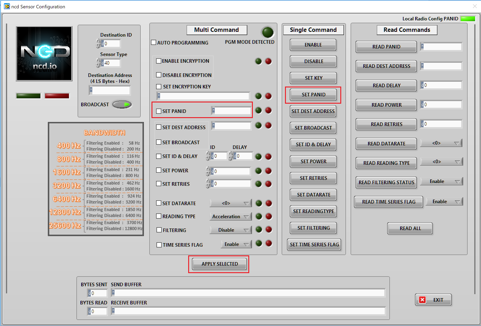
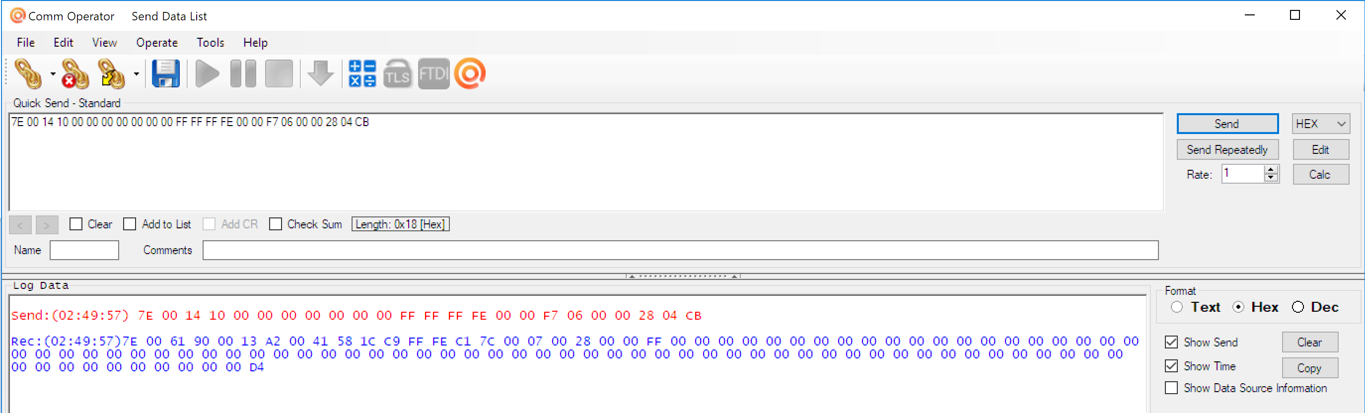
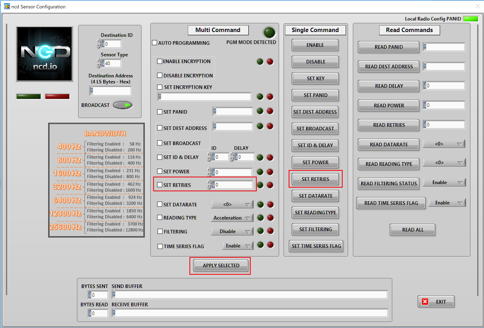
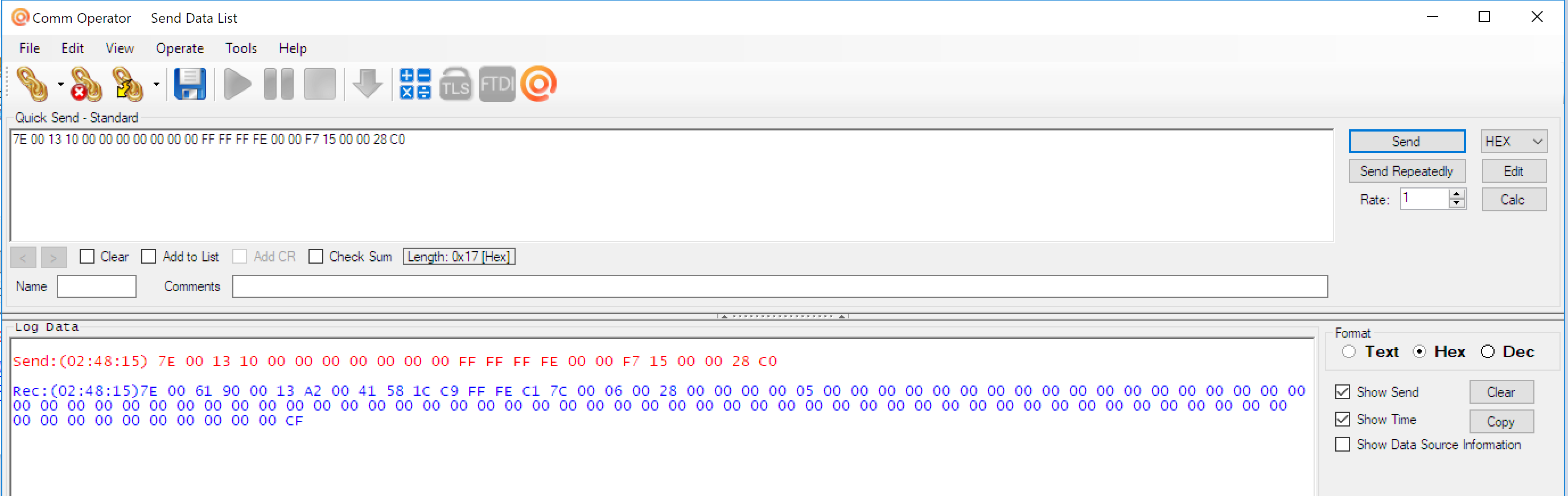
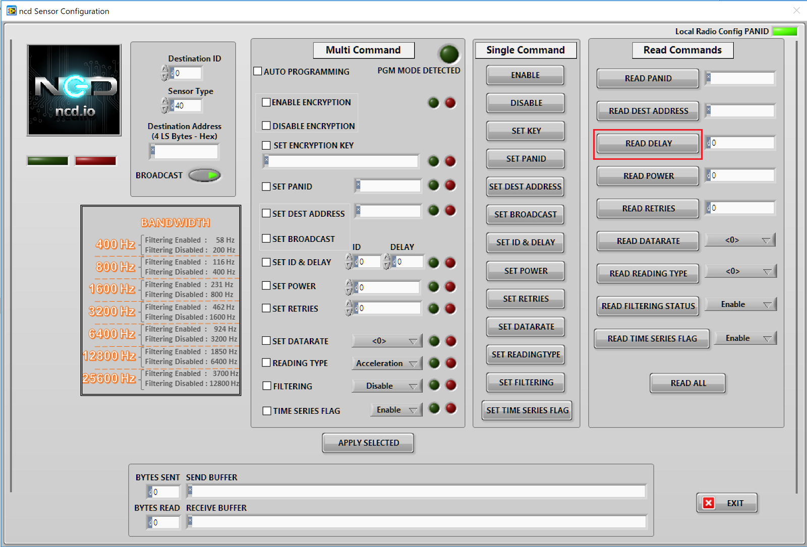
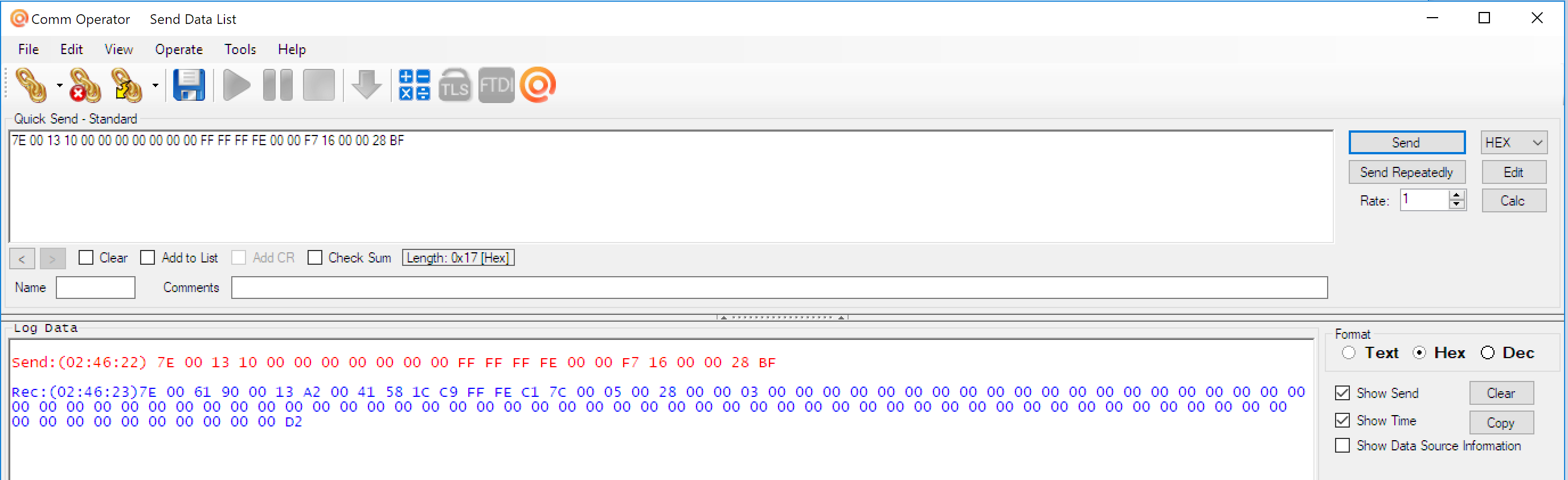
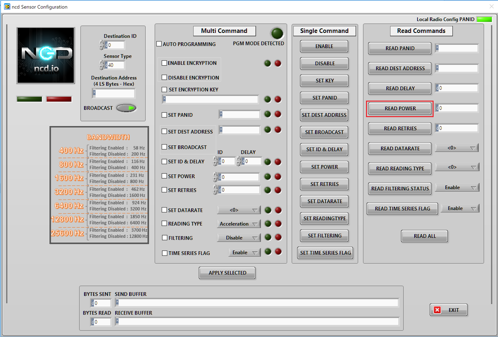
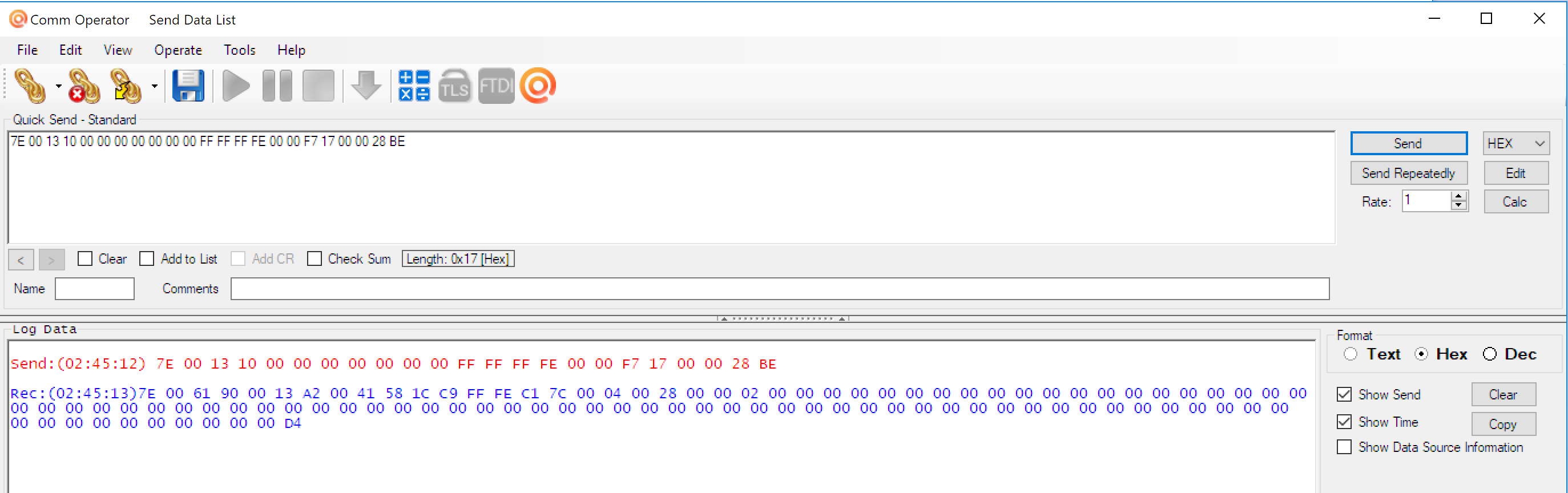
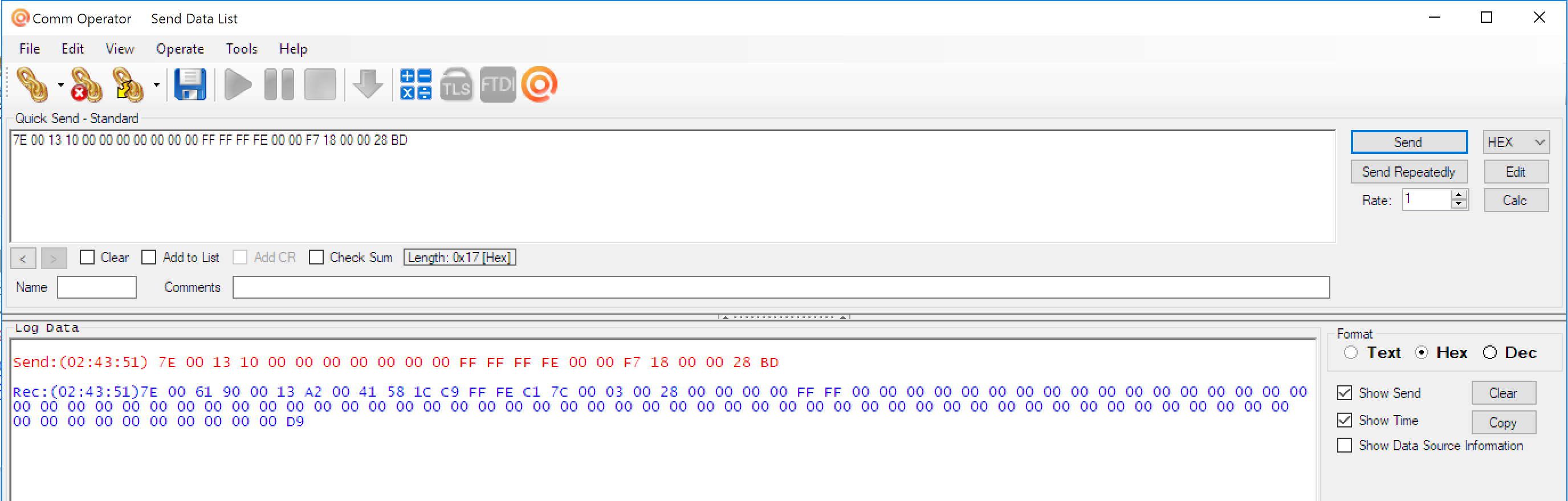
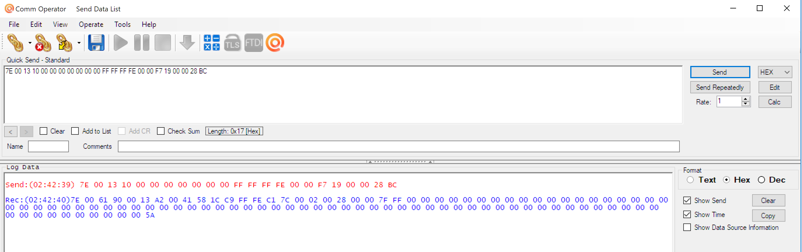
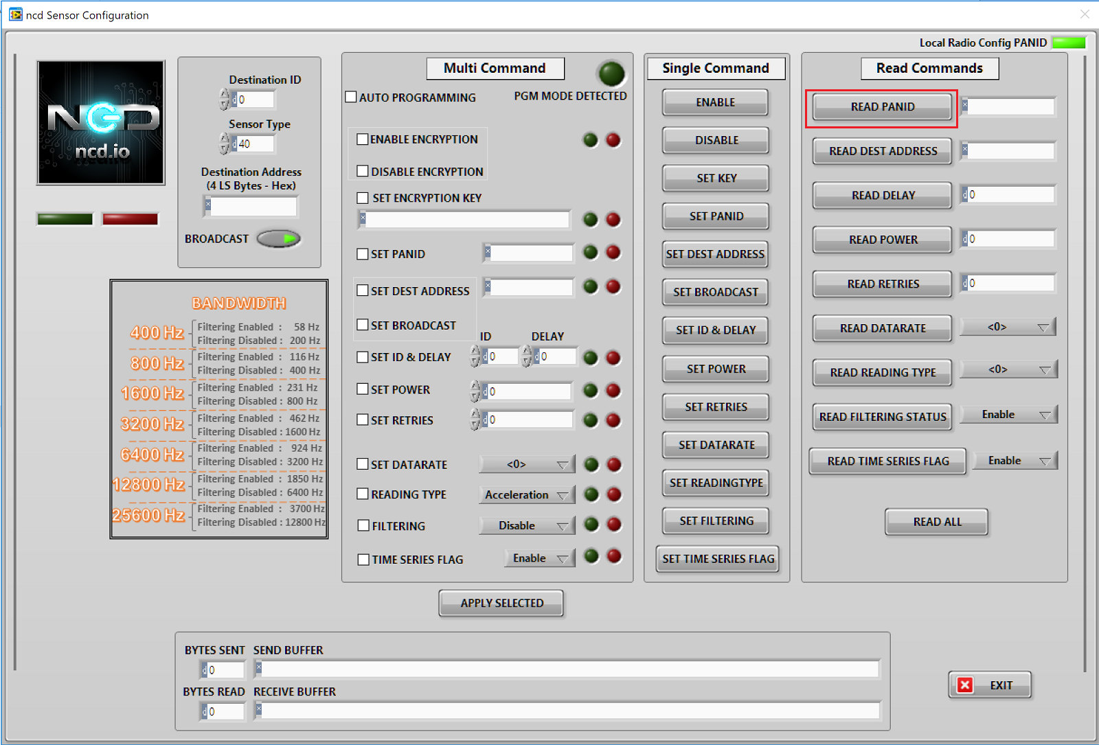
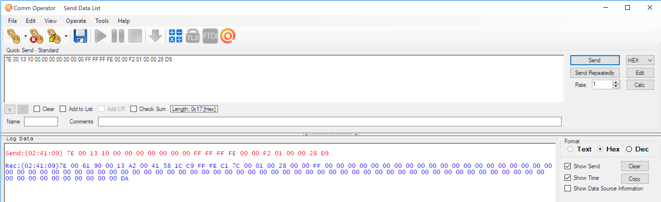
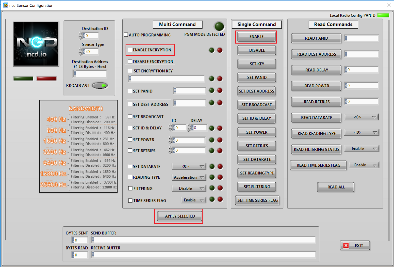
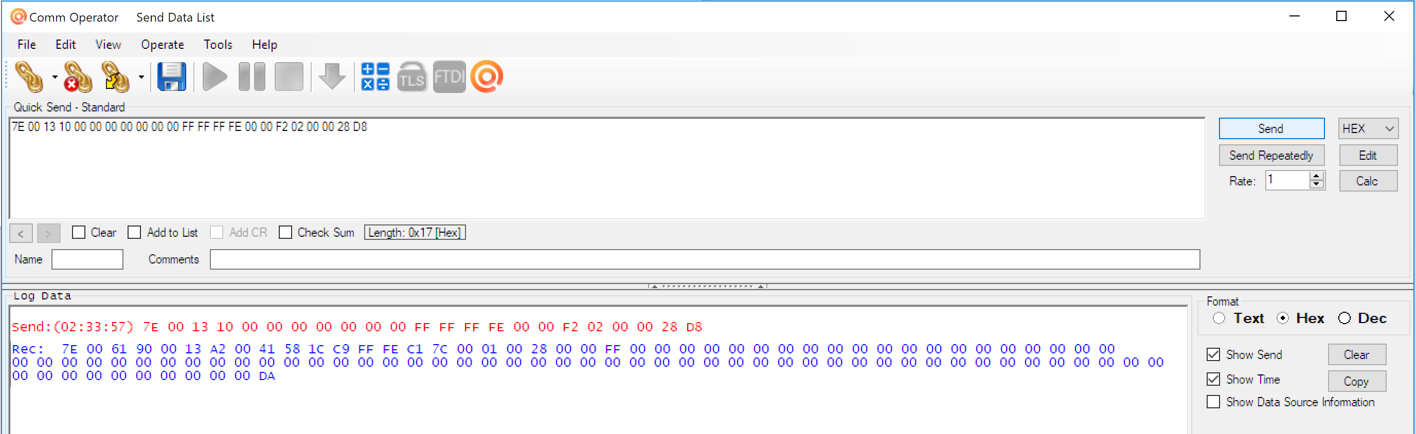
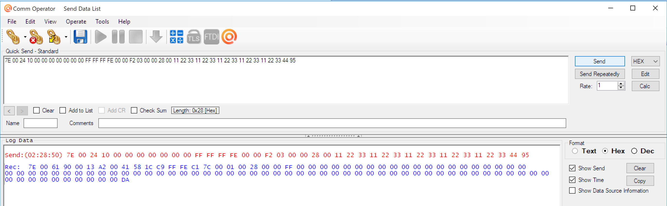
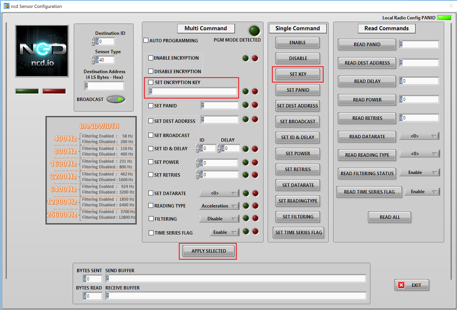
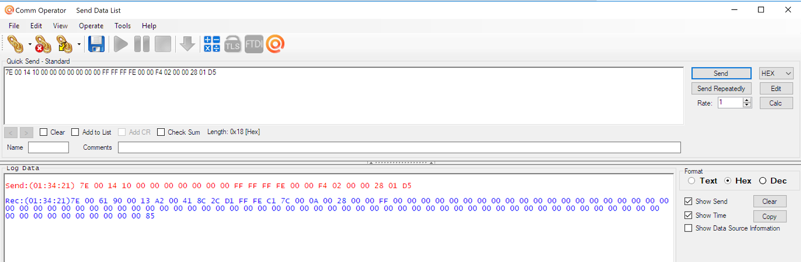
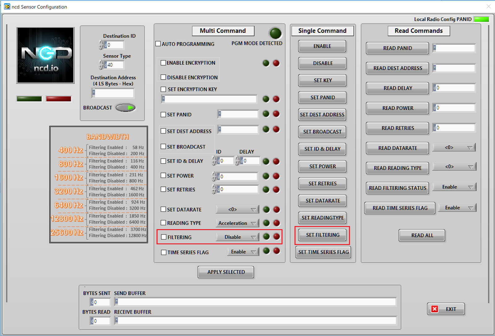
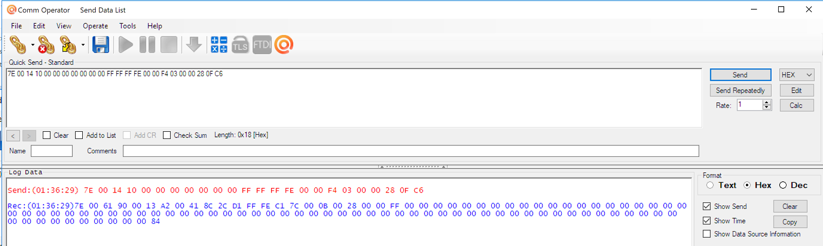
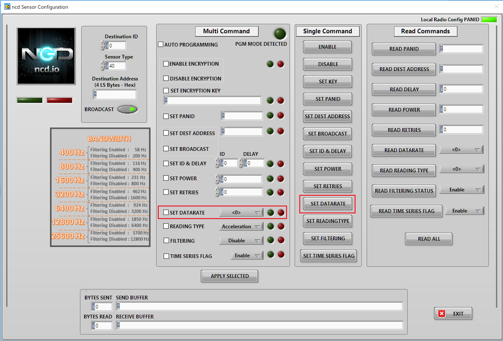
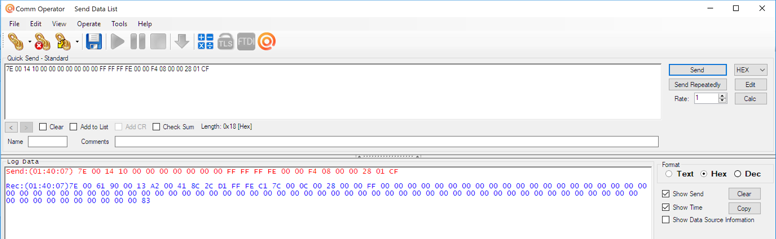
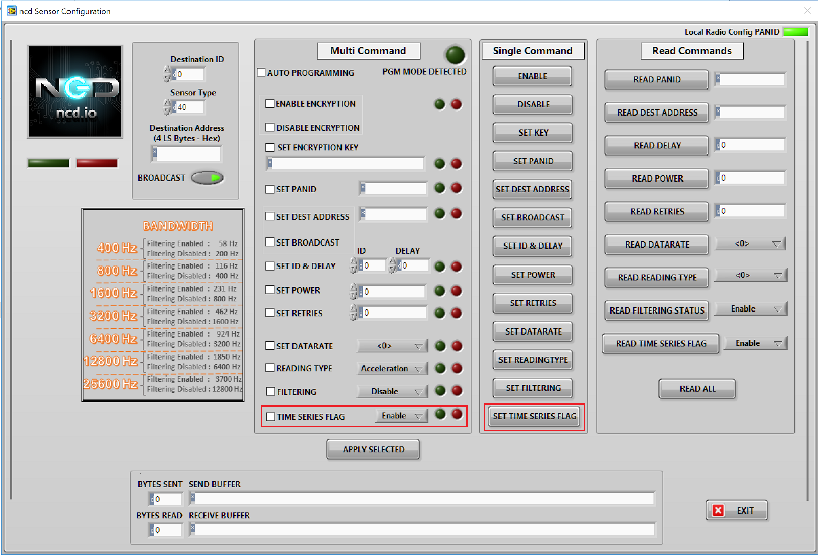
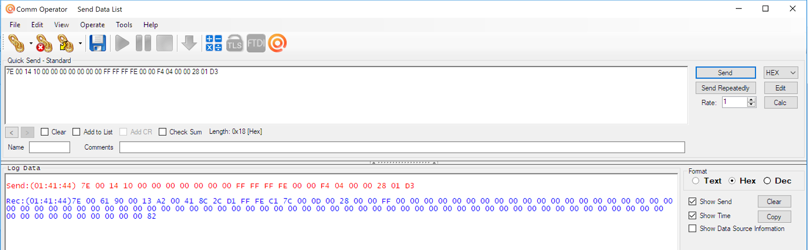
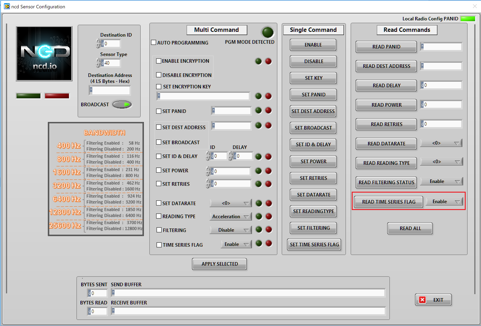
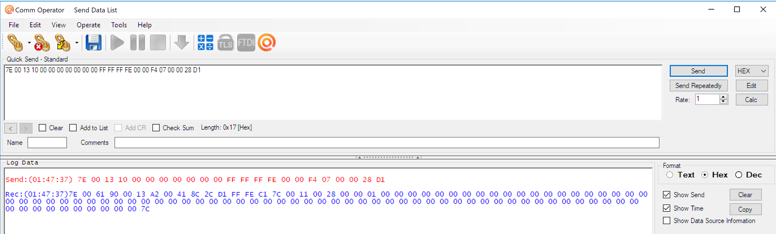
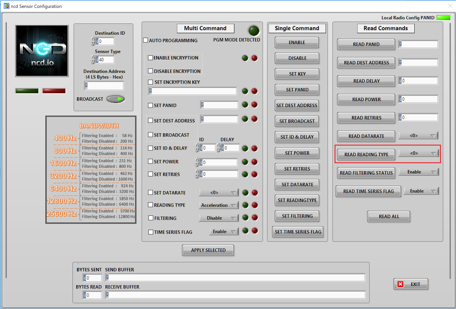
With an open communication protocol this sensor can be integrated with just about any control system or gateway. Data can be transmitted to a PC, a Raspberry Pi, to Microsoft Azure® IoT, or Arduino. Sensor parameters and wireless transmission settings can be changed on the go using the open communication protocol providing maximum configuration depending on the intended application.

The range, price, accuracy, battery life and security features of Enterprise Wireless Vibration Sensor makes it an affordable choice which exceeds the requirements for most of the Industrial as well as consumer market applications.

To complete a network with an industrial sensor at one end, a Zigmo/Router is required at the receiving end (PC end) that receives data from sensor. A set of sensor and Zigmo is shown in following figure.

Sensor with Zigmo/Router

Getting Started

The Vibration Sensors  and Zigmo/Router come pre-programmed and work out of the box. In this section we will setup a sensor and Zigmo link and start receiving data on our PC. Though this guide shows how to visualize data on LabVIEW utility, you can also use a simple serial terminal to see raw data by following these steps.

Resources Required

Note: The Wireless Sensor comes with external power enabled, for battery conservation during shipping. To enable battery power, open the enclosure and set the PS (power select) jumper which is parallel to the marking line on the board.

Steps

  1.  Power-up the Wireless Sensor and make sure its antenna is installed
  2. Connect your Zigmo/Router to your PC
Figure 1: Connect Zigmo/Router to PC
  1. Identify the serial port allocated to it by going into device manager (You can also find the serial port using Digi provided utility XCTU)
At this stage, both the Sensor and Zigmo have automatically established communication and the data can be read from the serial port at which Zigmo has been installed.
Figure 2: Serial port identification
  1. Install the LabVIEW utility for the sensor you are working with. Run this utility.
  2. Press the port configure button and select the PORT you identified in step 3. Select baud rate of 115200 and press OK.
Figure 3: LabVIEW Utility for Sensor
  1. Press the Run button to visualize incoming data.

If you were not able to communicate after completing the above steps then there might be a fault at either end of the communication network. Please refer to the troubleshooting section for identifying and resolving some common issues. If you are still not able to communicate after troubleshooting then please contact us at any time.

Figure 4: LabVIEW Utility for sensor showing incoming data

Troubleshooting

Changed/Unknown setting at sensor end

One of the issues for unsuccessful communication can be a changed setting at the sensor end due to which the sensor and Zigmo are unable to establish a connection. You can resolve this problem by going back to the factory default settings which are provided in Table 1. Please refer to Figure 7 and follow steps shown in it for applying factory default settings.

Once the sensor resets it will start sending a frame every 600 seconds after factory reset.

Please refer to the detailed document available to Digi website to understand X-bee communication parameters and its operation mechanism.

Table 1: Default Parameters programmed after Factory reset sequence

Changed/Unknown setting at PC end

Sometimes a changed setting at Zigmo end, whether intentional or unintentional, can cause a network failure and no data reception at PC end. To fix this issue when the sensor end is operating at factory default settings you will have to bring the Zigmo/Router to factory default settings as well. For that, please download the configuration file for Zigmo from our website. You will also require XCTU utility provided by Digi.

After installing XCTU Utility, run it and go to add a radio module. Select the serial port at which Zigmo is connected and press finish. This will connect the Zigmo to XCTU.

Figure 5: Connecting Zigmo/Router to XCTU

After double clicking the added module, a list of parameters will be displayed on the right side. Select the load configuration file from the top and select configuration file form the location where you downloaded it earlier.

Now press the write button on top to write these parameters. Close the XCTU utility and open the LabVIEW utility and follow the steps in getting started section to communicate with sensor.

Figure 6: Loading a default profile to Zigmo/Router

Modes of Operation

This module incorporates 2 modes of operation, these are

  • Run Mode
  • Configuration Mode


Run mode is the standard mode, the module will always enter Run mode if no button is pressed during Power-up/Reset. Configuration mode is intended to configure sensor parameters and the X-bee parameters on the sensor end. Note that the Sensor end X-bee is only configurable via the sensor controller using the commands provided in device manual. Figure 7 illustrates these modes.

The device sends a startup packet which can be used to determine the mode in which it is operating. These packets are shown in Table 2.

Mode Selection Process

The CFG button on the module is used to change mode. If CFG button is pressed and the module reset button is pressed, the module will enter the configuration mode. The amount of time CFG button has to be pressed is shown in Figure 7.

Note that settings only take effect after the reset.

Figure 7: Mode Selection Process
Frame Communication at Power up

In figure 8,  Mode bytes highlighted in red can be compared with the values provided in Table 2 to determine the mode in which the sensor is operating. Node ID is the ID of the given sensor while sensor type determines the type of sensor. Both of these can be used to determine the exact sensor which is sending the information.

A shown in second column in Table 2, the sensor configures its PAN ID automatically depending upon the mode it is working in. During factory reset it sets the PAN ID to the value given in table therefore the factory reset frame will only be received if your Zigmo/Router PAN ID matches this ID. Please note that right after factory reset the sensor enters configuration mode therefore its PAN ID is changed again and a new frame is generated. All 3 type of frames are shown in Figure 9, Figure 10 and Figure 11.


The factory default settings are shown in Table 1. For parameter description please refer to the section on configuration.

Table 2: Mode Bytes for different sensor modes (* this frame is followed by configuration frame as shown Figure 7)
Figure 8: Typical Communication at Power Up, Transmitted packet (left) Received packet (right)
Figure 9: Run Mode Power up frame
Figure 10: Configuration Mode Power up frame
Figure 11: Factory Default Power up frame

Run Mode

Standard Data Transmission

Standard data transmission mode is the default mode of operation of this sensor. In this mode the sensor sends periodic packets to destination receiver. During the time it is not sending packets, it sleeps and conserves power. Sensor end X-bee operates in API mode and sends packets to the saved destination address on the network specified by the saved PAN ID. Figure 12 illustrates an API packet transmission and reception.

Packet reception at receiver end is ensured by the device by retrying up to 3 times if no acknowledgement is received that the packet has been successfully received. The device uses the acknowledgement functionality available in API mode in X-bee devices therefore user does not need to worry about sending acknowledgements for every packet.

Figure 12: Transmit packet detail (left), Received packet detail (right)

The detail for API packet received at PC end can be read from the X-bee manual available from Digi. The detail of Payload section of packet is shown in Table 3.

Typical response from the device in Standard data transmission mode is shown in Figure 13 and Figure 14. The utility shown in Figure 14 can be downloaded from the website.

Table 3: Packet payload field and its description

The detail for API packet received at PC end can be read from the X-bee manual available from Digi. The detail of Payload section of packet is shown in Table 3.

Typical response from the device in Run mode is shown in Figure 13 and Figure 14. The utility shown in Figure 14 can be downloaded from the website.

Frame FieldOffset (Payload Section)Fixed Value
(if any)
Description
Header00x7F
Header to differentiate various type of packets
Node ID10x00 Factory Default
Node ID to differentiate up to 256 nodes in a network. User configural values
Firmware2
Used to determine firmware version programmed in the device
Battery VoltageMSB 3

Sampled battery voltage of the device.

Battery Voltage=((Battery Voltage MSB x 256+Battery Voltage LSB) x 0.00322 V

LSB 4
Packet Counter5
It is an 8-bit counter that increments with each packet transmission. It can be used to detect missing packets.
Sensor TypeMSB 60x00
Two bytes to determine sensor type. It can be used in conjunction with Node ID to create sensor networks of up to 256 nodes for a single type of sensor and multiple such networks can coexist and can be differentiated in processing software on PC end
MSB 70x28
Status (b :bit)80x00

Sensor Status as defined below, shift the status bit right 2 places for the integer value (b >> 2), the value in parentheses is there for completeness and is consistent with the data sheet.

Decimal Value

[b7-b2]

Status
0Valid
63 (-1)

Invalid Argument

62 (-2)Internal sensor communication failure
61 (-3)Invalid sensor discovery
60 (-4)Invalid length
59 (-5)ASIC test failure
58 (-6)Device initialization failure
57 (-7)Soft-reset failure
b1

Data Type in Payload defined by following:

1: Acceleration (g)

2: Velocity (inch/sec)

3: Time domain data (acceleration in g)

b0(LS)
Vibration RMS9/X[0]

Vibration RMS X-axis Data (24 bit Signed Output)

          Vibration (mg) = ((X[0]<<16)+(X[1]<<8)+X[2])/100

(Saving directly to 32bit integer will give wrong result

10/X[1]
11/X[2]
12/Y[0]

Vibration RMS Y-axis Data (24 bit Signed Output)

          Vibration (mg) = ((Y[0]<<16)+(Y[1]<<8)+Y[2])/100

(Saving directly to 32bit integer will give wrong result

13/Y[1]
14/Y[2]
15/Z[0]

Vibration RMS Z-axis Data (24 bit Signed Output)

          Vibration (mg) = ((Z[0]<<16)+(z[1]<<8)+Z[2])/100

(Saving directly to 32bit integer will give wrong result

16/Z[1]
17/Z[2]
Vibration Max18/X[0]

Vibration Max X-axis Data (24 bit Signed Output)

          Vibration (mg) = ((X[0]<<16)+(X[1]<<8)+X[2])/100

(Saving directly to 32bit integer will give wrong result

19/X[1]
20/X[2]
21/Y[0]

Vibration Max Y-axis Data (24 bit Signed Output)

          Vibration (mg) = ((Y[0]<<16)+(Y[1]<<8)+Y[2])/100

(Saving directly to 32bit integer will give wrong result

22/Y[1]
23/Y[2]
24/Z[0]

Vibration Max Z-axis Data (24 bit Signed Output)

          Vibration (mg) = ((Z[0]<<16)+(Z[1]<<8)+Z[2])/100

(Saving directly to 32bit integer will give wrong result

25/Z[1]
26/Z[2]
Vibration Min27/X[0]

Vibration Min X-axis Data (24 bit Signed Output)

          Vibration (mg) = ((X[0]<<16)+(X[1]<<8)+X[2])/100

(Saving directly to 32bit integer will give wrong result

28/X[1]
29/X[2]
30/Y[0]

Vibration Min Y-axis Data (24 bit Signed Output)

          Vibration (mg) = ((Y[0]<<16)+(Y[1]<<8)+Y[2])/100

(Saving directly to 32bit integer will give wrong result

31/Y[1]
32/Y[2]
33/Z[0]

Vibration Min Z-axis Data (24 bit Signed Output)

          Vibration (mg) = ((Z[0]<<16)+(Z[1]<<8)+Z[2])/100

(Saving directly to 32bit integer will give wrong result

34/Z[1]
35/Z[2]
Temperature Data36/T[0]

 Temperature data (16 bit Signed Output)

          Temperature (°C) = (T[0]<<8)+T[1]

37/T[1]
Figure 13: Run mode packets being received in a terminal (Hex mode)
Figure 14: Run mode packets being received in our free to use LabVIEW utility (For custom made utility for your specific requirements please contact support)
Time domain data transmission

The Enterprise Wireless Vibration Sensor enables time domain data to be downloaded from the sensor. This enables a vibration analyst to dig deep into the root cause by processing time domain data and analyzing it in both time and frequency domains. The sampling rate and bandwidth can be configured according to the frequency bin resolution and the range of frequencies to be analyzed in the frequency analysis.

The time domain data can only be queried using the command(in hex) shown below:

7E00 1310 0000 0000 0000 00FF FFFF FE00 00F8 9900 0028 3B

As mentioned earlier, the sensor goes back to sleep after successfully sending standard data transmission packet. However, if TIME SERIES flag is enabled from the configuration mode, the sensor waits an additional 600msec to wait for the time series command. If the above command is received during this interval, it sends out time domain data and goes back to sleep. Note that, the sensor power consumption is increased if time series flag is enabled.

Time domain data comprises of 340 samples for each axis. Each sample is a 16-bit integer. Hence, total time domain data contains 2040 bytes. Due to the limitation of packet size for X-bee communication, this data is segmented and sent in 12 packets as shown in following figure. Data has to be recombined at the receiver end into 340 samples for each axis before further processing. It should be noted that since the amount of data is big therefore it is only sent on demand and at the destination address saved inside the sensor. For this purpose, the source address from the packet containing command is matched with the saved destination address. This step essentially verifies that the command is coming from designated node. If, however, the destination address stored inside the sensor is a broadcast address, then this matching is disabled and the time domain data is sent to all listening nodes.

 
Figure 15: Time domain data packets detail

The 2 byte data samples are integer counts of the acceleration and must be converted into acceleration unit(g) by dividing the count value with 2048 since 1 count equals 0.488mg. The following Figure shows a User Interface that display time domain data on the left side and its Fast Fourier Transform (FFT) on the right side.

Figure 16: Time domain data reception, display and frequency domain analysis (FFT)
RMS Noise for various bandwidth settings

Following figure illustrates the RMS noise present in sensor acquired data against various bandwidth settings.

Table 4: Configurable Bandwidth Settings
Figure 17: RMS Noise for various Bandwidth settings and comparison

Configuration Mode

Configuration mode is intended to setup the device over the wireless link. Entering configuration mode was already explained in the section “mode selection procedure”. User can also setup X-bee communication and networking parameters using this mode via PC. Note that settings only take effect after reset and are stored inside the device.

In configuration mode, the device sets its X-bee pan id to 7BCD (Hex). Also, the destination address used by the sensor is extracted from the incoming packet (source address). This ensures that once you put a device in configuration mode you just need to change the PAN ID of your Zigmo to match with sensor and start configuring your device. You can change the PAN ID of your Zigmo using XCTU from Digi. If you use our LabVIEW utility, it will automatically change Zigmo PAN ID once you open the configuration window. When you exit this window your PAN ID will be restored to old value.

A standard configuration packet and its fields are explained in Figure 18. Its possible responses are also shown. The commands supported by this sensor are shown in Table 5, these can be used in the Parameters field of Payload section. The sensor responds to these commands with an acknowledgement if the process completed successfully or with an error if it failed to setup a parameter. The respective Data and Reserve section length and values are shown in Table 6 for the case of acknowledgement. In the case of error, the reserved section will be fixed and not used, while the Error number byte will determine the type of error returned. These errors are mentioned in Table 7.

Figure 18 depicts standard communication between Zigmo/Router and sensor. Sensor commands have variable length frames whereas responses received from sensor are fixed length. The 2 scenarios are also shown, where a command can result in an acknowledgement reception or an error reception at the Zigmo end.

The Configuration mode also supports 6-point calibration to improve the accuracy of the results by determining 0-g offsets and sensitivities for each axis. The command to initiate 6-point calibration is provided in the table below. The response received from the sensor is in ASCII text and self explanatory. To advance the calibration process, GO command is required to be sent to the sensor which is also described in the table below. 

Examples for setting parameters in configuration mode are shown in Appendix A. Note that incorrectly setting some of the critical settings such as setting PANID and Destination address can disable further communication between a Zigmo and the sensor. Hence, these settings are saved in the sensor but they take affect after a reset so that the communication is not lost.

Figure 18: Configuration mode communication
Table 5: Configuration Commands and their respective headers, sub command and Parameter field

The sensor has 4 time domain data modes
1. No time domain
sample complete API packet
7E 00 14 10 00 00 00 00 00 00 00 FF FF FF FE 00 00 F4 08 00 00 28 01 CF
Command — F4 08 00 00 28 01
2. Only time domain data
7E 00 14 10 00 00 00 00 00 00 00 FF FF FF FE 00 00 F4 08 00 00 28 02 CE
Command — F4 08 00 00 28 02
3. Time domain data with each packet
7E 00 14 10 00 00 00 00 00 00 00 FF FF FF FE 00 00 F4 08 00 00 28 03 CD
Command — F4 08 00 00 28 03

4. Time domain on demand (This command needs to be sent within 1 sec of data reception)
7E 00 14 10 00 00 00 00 00 00 00 FF FF FF FE 00 00 F4 08 00 00 28 04 CC
Command — F4 08 00 00 28 04

Once the gateway receives the data, it needs to send a command to request on demand time domain data

7E 00 13 10 01 00 00 00 00 00 00 FF FF FF FE 00 00 F8 99 00 00 28 3A

Command —  F8 99 00 00 28

F8 — Command Header

99 — Sub command

00 — node id

00,28 — Sensors type

Once the sensor gets this command it will send RMS, Max,Min, vibration data plus the time domain data

Table 6: Acknowledgment data for various commands and the size of reserve section in each case
Table 7: Error numbers and their description

The UI, shown in Figure 19, can be used to configure the wireless sensor. At startup, it automatically changes the Zigmo PANID so that it can communicate with a sensor in configuration mode (indicated by the Led on the top right). Upon exit, the PANID of the Zigmo is restored to old value.

Individual settings can be programmed using the single command column.
The AUTO PROGRAMMING check option allows the user to setup multiple sensors with the same settings. In such a scenario, the user will be required to enable each check box for enabling a setting, enter the value for each setting if required and then check the auto programming check box. Afterwards, when a sensor is powered up and enters configuration mode, the PGM MODE DETECTED Led will flash and automatically program the checked settings. User can also program multiple settings by clicking the APPLY SELECTED button. Moreover, settings can be read using the individual buttons or all settings can be read using the READ ALL button.


Figure 19: Configuration mode User Interface

Appendix A

Configuration Commands

1. Set Broadcast Transmission

Command For COPY: 7E00 1310 0000 0000 0000 00FF FFFF FE00 00F7 0100 0028 D4

2. Set ID and Delay

Command For COPY: 7E00 1710 0000 0000 0000 00FF FFFF FE00 00F7 0200 0028 0000 0005 CE

3. Set Destination Address

Command For COPY: 7E00 1710 0000 0000 0000 00FF FFFF FE00 00F7 0300 0028 1234 5678 BE

4. Set Power

Command For COPY: 7E00 1410 0000 0000 0000 00FF FFFF FE00 00F7 0400 0028 03CE

5. Set PANID

Command For COPY: 7E00 1510 0000 0000 0000 00FF FFFF FE00 00F7 0500 0028 7CDE 76

6. Set Retries

Command For COPY: 7E00 1410 0000 0000 0000 00FF FFFF FE00 00F7 0600 0028 04CB

7. Read Delay

Command For COPY: 7E00 1310 0000 0000 0000 00FF FFFF FE00 00F7 1500 0028 C0

8. Read Power

Command For COPY: 7E00 1310 0000 0000 0000 00FF FFFF FE00 00F7 1600 0028 BF

9. Read Retries

Command For COPY: 7E00 1310 0000 0000 0000 00FF FFFF FE00 00F7 1700 0028 BE

10. Read Destination Address

Command For COPY: 7E00 1310 0000 0000 0000 00FF FFFF FE00 00F7 1800 0028 BD

11. Read PANID

Command For COPY: 7E00 1310 0000 0000 0000 00FF FFFF FE00 00F7 1900 0028 BC

12. Enable Encryption

Command For COPY: 7E00 1310 0000 0000 0000 00FF FFFF FE00 00F2 0100 0028 D9

13. Disable Encryption

Command For COPY: 7E00 1310 0000 0000 0000 00FF FFFF FE00 00F2 0200 0028 D8

14. Set Encryption Key

Command For COPY: 7E00 2410 0000 0000 0000 00FF FFFF FE00 00F2 0300 0028 0011 2233 1122 3311 2233 1122 3311 2233 4495

15. Set Filtering

Command For COPY: 7E00 1410 0000 0000 0000 00FF FFFF FE00 00F4 0200 0028 01D5

16. Set Data Rate

Command For COPY: 7E00 1410 0000 0000 0000 00FF FFFF FE00 00F4 0300 0028 0FC6

17. Set Time Series Flag

Command For COPY: 7E00 1410 0000 0000 0000 00FF FFFF FE00 00F4 0800 0028 01CF

18. Set Reading Type

Command For COPY: 7E00 1410 0000 0000 0000 00FF FFFF FE00 00F4 0400 0028 01D3

19. Read Filtering

Command For COPY: 7E00 1310 0000 0000 0000 00FF FFFF FE00 00F4 0500 0028 D3

20. Read Data Rate

Command For COPY: 7E00 1310 0000 0000 0000 00FF FFFF FE00 00F4 0600 0028 D2

21. Read Time Series Flag

Command For COPY: 7E00 1310 0000 0000 0000 00FF FFFF FE00 00F4 0900 0028 CF

22. Read Reading Type

Command For COPY: 7E00 1310 0000 0000 0000 00FF FFFF FE00 00F4 0700 0028 D1

Appendix B

Frame Checksum Calculation

In order to successfully communicate over the API protocol, checksum is of vital importance. The X-bee at either end will reject packets if the checksum is not matched. Checksum is also checked by the sensor controller and LabVIEW utility for added security.

For sending packets, checksum calculation works as follows

  1. Add all the bytes and keep the lower 8 bits of result (Excluding the frame delimiter and length)
  2. Subtract this value from 0xFF (hex)
  3. The resultant value is the checksum
  4. Append this byte at the end of the original packet for sending

Consider the example for the command Set Broadcast shown in Figure 19 in A APPENDIX and see that the calculated checksum matches with the checksum sent by the terminal/LabVIEW

Although checksum is matched by the X-bee itself, but for understanding follow these steps to match checksum at reception

  1. Add all the bytes including the received checksum (Exclude the frame delimiter and length)
  2. Keep only the last 8 bits
  3. If the result is 0xFF, the checksum is correct and the packet can be processed.

Consider the example of the command Set Broadcast shown in Figure 19 in A APPENDIX and see that the received packet checksum verifies since the result is 0xFF.